About these slides
- Goal is the least that you need to know
- All slides are created in Jupyter notebooks - free to use and open source
- Github repo
- pyglide provides the interactivity
Part 2 Measurement
Measurement
- Key principle: repeatability - if you measure a subject twice do you get the same value
- Key principle in measuring repeatability: compare intra-subject variation to inter-subject variation
- Repeatability is relatively easy to measure, since we can take technical replicates
- Repeatability does not measure validity, the extent to which a measure actually measures what it's reported to
In [4]:
## Code used to generate figures
import part2_code
Low inter-subject variability to intra-subject variability
In [ ]:
part2_code.measurement1()

High inter-subject variability to intra-subject variability
In [ ]:
part2_code.measurement2()

ICC
- The intra-class correlation coefficient is a measure of repeatability
- ICC is the proportion of the total variability that is inter-subject
- Note the inter-subject varability is dependent on the sample characteristics
- Suppose older subjects tend to have higher mean values
- A sample of older and younger subjects will have more inter-subject variability than one of just older subjects or just younger subjects alone
Estimation
- Usually estimation follows by random effect models; we'll show the basics
- $i$ = subject; $j$ = measurement within subject (assume $j=1,2$)
- $U_i$ is the effect of subject $i$; variation in $U_i$ is inter-subject variation, $\sigma^2_u$
- $\epsilon_{ij}$ is the error; variation in $\epsilon_{ij}$ is intra-subject variation, $\sigma^2$
Estimation continued
- Notice that: $$Y_{i2} - Y_{i1} = \epsilon_{i2} - \epsilon_{i1}$$
- Implying $$Var(Y_{i2} - Y_{i1}) = 2\sigma^2$$
- And also that: $$\frac{1}{2}(Y_{i2} + Y_{i1}) = U_i + \frac{1}{2}(\epsilon_{i2} + \epsilon_{i1})$$
- Implying $$Var\left[\frac{1}{2}(Y_{i2} + Y_{i1})\right] = \sigma_u^2 + \frac{\sigma^2}{2}$$
Estimation continued
- So we can get: $$\frac{1}{2} Var(Y_{i2} - Y_{i1}) = \sigma^2$$
- And : $$Var\left[(\frac{1}{2}(Y_{i2} + Y_{i1})\right] - \frac{\sigma^2}{2} = \sigma^2_u$$
Example measuring CSF
- Below we show repeated measurements of human brain ventricle size on 20 subjects
- We first show a scatterplot then a so-called Tukey mean/difference plot, also called a Bland/Altman plot
Reading in the data
In [ ]:
import pandas as pd
import matplotlib.pyplot as plt
visit1 = pd.read_csv("assets/visit1_mricloud.csv")
visit2 = pd.read_csv("assets/visit2_mricloud.csv")

csf1 = visit1[(visit1['Type'] == 1) & (visit1['Level'] == 1)
              & (visit1['Object'] == 'CSF')]['Volume']
csf2 = visit2[(visit2['Type'] == 1) & (visit2['Level'] == 1)
              & (visit2['Object'] == 'CSF')]['Volume']
plt.scatter(csf1, csf2);

In [ ]:
import statsmodels.api as sm
sm.graphics.mean_diff_plot(csf1, csf2)
plt.show()

In [ ]:
import numpy as np
sm.graphics.mean_diff_plot(np.log(csf1), np.log(csf2))
plt.show()

In [ ]:
## Calculating the ICC manually
sigmasq = np.var(np.log(csf1) - np.log(csf2))
sigmausq = np.var(0.5 * np.log(csf1) + 0.5 * np.log(csf2)) - sigmasq/2
print(100 * sigmausq / (sigmausq + sigmasq))
98.84502763511378
Notes
- This is not how one typically estimates ICC anymore; mixed models are typically used
- The subtraction can result in a negative variance estimate
In [ ]:
#### Fitting the random effect model
import pingouin as pg
import statsmodels.formula.api as smf

csfdf1 = visit1[(visit1['Type'] == 1) & (visit1['Level'] == 1)
                & (visit1['Object'] == 'CSF')]
csfdf2 = visit2[(visit2['Type'] == 1) & (visit2['Level'] == 1)
                & (visit2['Object'] == 'CSF')]

csfdf = pd.concat( [csfdf1, csfdf2] )
csfdf['logvolume'] = np.log(csfdf['Volume'])
md = smf.mixedlm("logvolume ~ 1", csfdf, groups=csfdf["ID"]).fit()
md.summary()
Out[ ]:
| Model: | MixedLM | Dependent Variable: | logvolume |
| No. Observations: | 38 | Method: | REML |
| No. Groups: | 19 | Scale: | 0.0003 |
| Min. group size: | 2 | Log-Likelihood: | 41.9000 |
| Max. group size: | 2 | Converged: | Yes |
| Mean group size: | 2.0 |
| Coef. | Std.Err. | z | P>|z| | [0.025 | 0.975] | |
|---|---|---|---|---|---|---|
| Intercept | 11.345 | 0.055 | 207.545 | 0.000 | 11.237 | 11.452 |
| Group Var | 0.057 | 1.491 |
Example
Calculation of ICC in the same example using the mixedlm function.
Final answer will be copied here
Example of repeatability studies
- In functional brain imaging one typically looks at the correlation in activity over time between brain regions
- These sets of correlations estimate how different areas of the brain coordinate
- Finn et al. (Nature Neuroscience 2015) used brain connectivity as a "fingerprint"
- They took pairs of measurements for subjects and found which measurements were the closest
- The count of the number of instances where a subject matched to themselves is a repeatability metric. They called it the "functional connectome fingerprint"
Fun fact
- In 1713 Montmort published his letters with Nicholaus Bernoulli
- In them he demonstrated that under independence, i.e. that fingerprints are being matched only by chance, the number of matches follows what is now called Montmort's matching distribution
- This distribution limits to a Poisson(1)
- Wang (2021, Canadian Journal of Statistics) showed that any reasonable matching strategy also limits to a Poisson(1)
- The convergence is quite fast
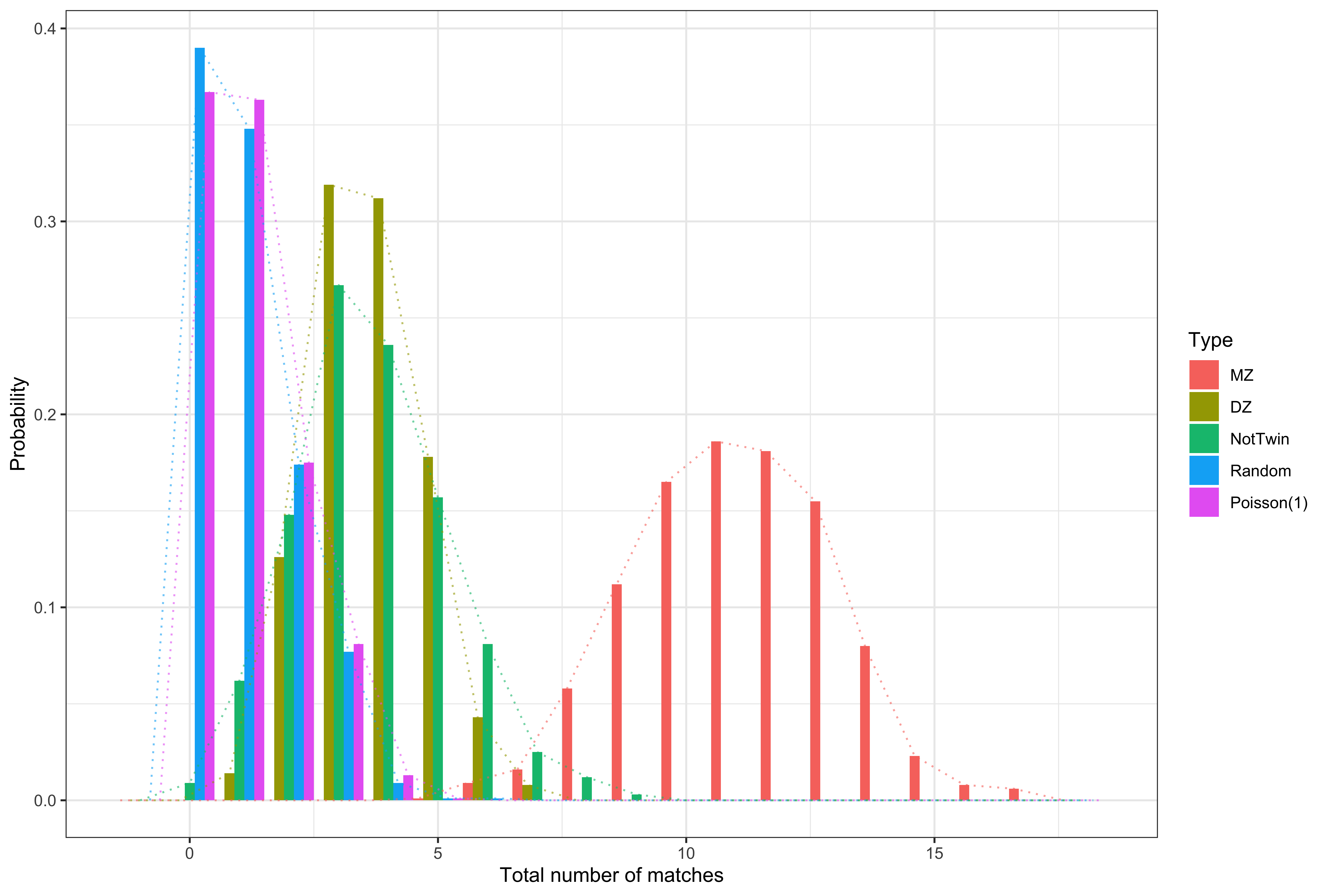
Courtesy of Wang et al. (2021 Canadian Journal of Statistics)
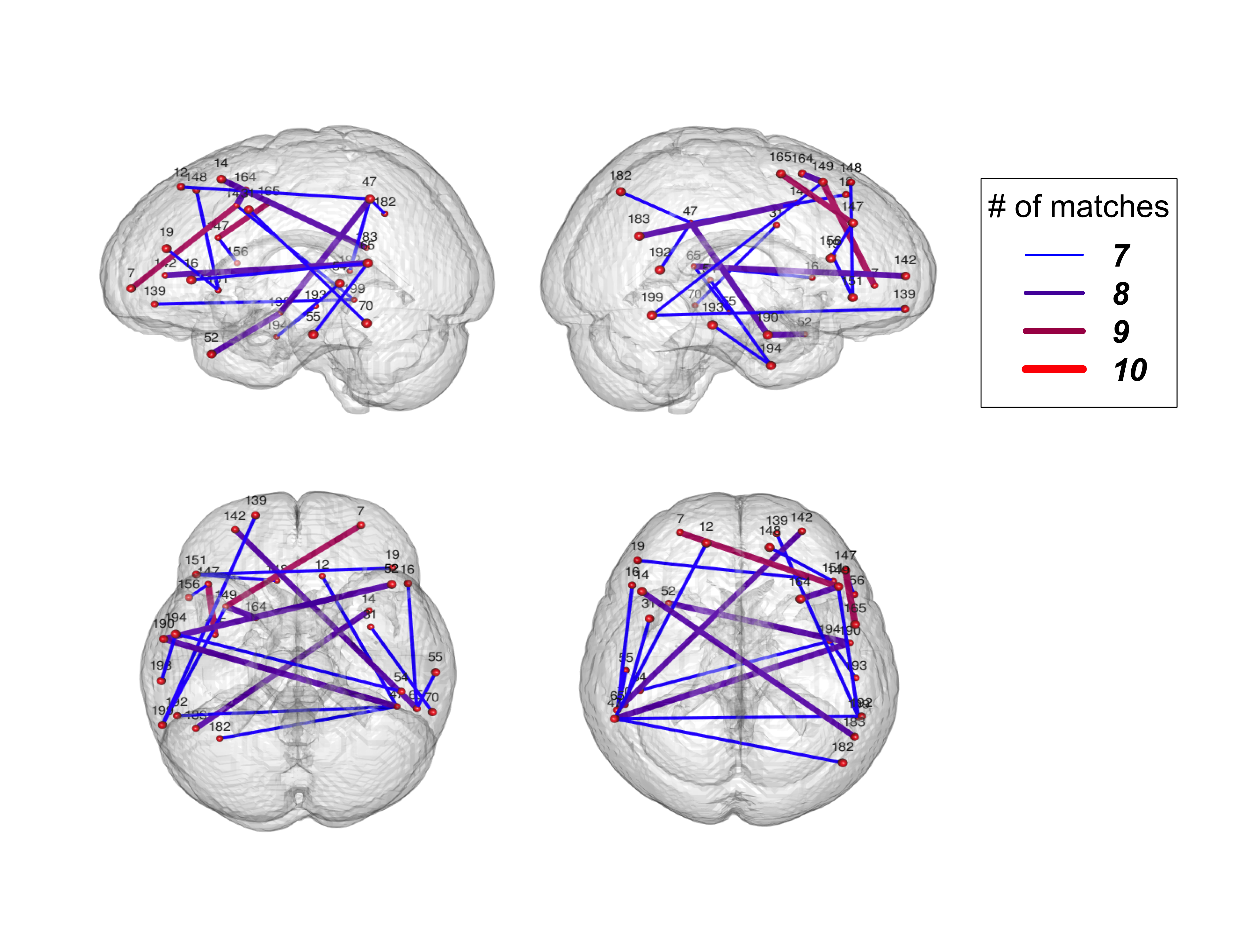
Courtesy of Wang et al. (2021 Canadian Journal of Statistics)
Validity
- Repeatability is not a measure of validity, that a construct measures what it purports to
- Repeatability is easy to measure, since we can collect technical replicates, observe units over short periods of time and so on
- Validity is often hard because the measurement we'd like to validate is the current best measure of the thing we'd like to estimate!
Things to try
- In the absence of a measurment gold standard, the statistical proceduer I find most useful is Predictive validity: is the measurement associated with outcomes that it should be?
- Also useful, concurrent validity is the measurement correlated with other measures of the target?
- Example: in a poor country where child ages are hard to determine due to poor record keeping an image based DL algorithm is used to estimate age.
- Repeatability - take different pictures of the same subject, do the predicted ages agree?
- Predictive validity - does the estimated age predict developmental milestones at roughly the right time
- Concurrent validity - is the estimated age correlated with height, weight and other measures of size