10  Unsupervised learning

10.1 PCA

Let \(\{X_i\}\) for \(i=1,\ldots,n\) be \(p\) random vectors with means \((0,\ldots,0)^t\) and variance matrix \(\Sigma\). Consider finding \(v_1\), a \(p\) dimensional vector with \(||v_1|| = 1\) so that \(v_1^t \Sigma v_1\) is maximized. Notice this is equivalent to saying we want to maximize \(\mathrm{Var}( X_i^t V_1)\). The well known solution to this equation is that \(v_1\) is the first eigenvector of \(\Sigma\) and \(\lambda_1 = \mathrm{Var}( X_i^t V_1)\) is the associated eigenvalue. If \(\Sigma = V^t \Lambda V\) is the eigenvalue decomposition of where \(V\) are the eigenvectors and \(\Lambda\) is a diagonal matrix of the eigenvalues ordered from greatest to least, then \(v_1\) corresponds to the first column of \(V\) and \(\lambda_1\) corresponds to the first element of \(\Lambda\). If one then finds \(v_k\) as the vector maximizing \(v_k^t \Sigma v_k\) so that \(v_k^t v_{k'} = I(k=k')\), then the \(v_k\) are the columns of \(V\) and \(v_k^t \Sigma v_k = \lambda_k\) are the eigenvalues.

Notice:

1. \(V \Sigma V^t = \Lambda\) (i.e. \(V\) diagonalizess \(\Sigma\))
2. \(\mbox{Trace}(\Sigma) = \mbox{Trace}(\Sigma V^t V) = \mbox{Trace}(V \Sigma V^t) = \sum \lambda_k\) (i.e. the total variability is the sum of the eigenvalues)
3. Since \(V^t V = I\), \(V\) is a rotation matrix. Thus, \(V\) rotates \(X_i\) in such a way that to maximize variability in the first dimension, then the second dimensions …
4. \(\mbox{Cov}(X_i^t v_k, x_i^t v_{k'} )= \mbox{Cov}(X_i^t v_k, x_i^t v_{k'} ) v_k^t \mbox{Cov}(x_i, x_i^t) v_{k'} = v_k^t V v_{k'} = 0\) if \(k\neq k'\)
5. Another representation of \(\Sigma\) is \(\sum_{k=1}^p \lambda_i v_k v_k^t\) by simply rewriting the matrix algebra of \(V \Lambda V^t\).
6. The variables \(U_i = V X_i\) then: have uncorrelated elements (\(\mbox{Cov}(U_{ik}, U_{ik'}) = 0\) for \(k\neq k'\) by property 5), have the same total variability as the elements of \(X_i\) (\(\sum_k \mbox{Var}(U_{ik}) = \sum_k \lambda_k = \sum_k \mbox{Var}(X_{ik})\) by property 2), are a rotation of the \(X_i\), are ordered so that \(U_{i1}\) has the greatest amount of variability and so on.

Notation:

1. The \(\lambda_k\) are simply called the eigenvalues or principal components variation.
2. \(U_{ik} = X_i^t v_k\) is called the principal component scores.
3. The \(v_k\) are called the principal component loadings or weights, with \(v_1\) being called the first principal component and so on.

Statistical properties under the assumption that the \(x_i\) are iid with mean 0 and variance \(\Sigma\)

1. \(E[U_{ik}]=0\)
2. \(\mbox{Var}(U_{ik}) = \lambda_k\)
3. \(\mbox{Cov}(U_{ik}, U_{ik'}) = 0\) if \(k\neq k'\)
4. \(\sum_{k=1}^p \mbox{Var}(U_{ik}) = \mbox{Trace}(\Sigma)\).
5. \(\prod_{k=1}^p \mbox{Var}(U_{ik}) = \mbox{Det}(\Sigma)\)

10.1.1 Sample PCA

Of course, we’re describing PCA as a conceptual process. We realize \(n\) \(p\) dimensional vectors \(x_1\) to \(x_n\), typically organized in \(X\) a \(n\times p\) matrix. If \(X\) is not mean 0, we typically demean it by calculating \((I- J(J^t J)^{-1} J') X\) where \(J\) is a vector of ones. Assume this is done. Then \(\frac{1}{n-1} X^t X = \hat \Sigma\). Thus, our sample PCA is obtained via the eigenvalue decomposition \(\hat \Sigma = \hat V \hat \Lambda \hat V^t\) and our principal components obtained as $ X V$.

We can relate PCA to the SVD as follows. Let \(\frac{1}{\sqrt{n-1}} X = \hat U \hat \Lambda^{1/2} \hat V^t\) be the SVD of the scaled version of \(X\). Then note that \[ \hat \Sigma = \frac{1}{n-1} X^t X = \hat V \hat \Lambda \hat V^t \] yields the sample covariance matrix eigenvalue decomposition.

10.1.2 PCA with a large dimension

Consider the case where one of \(n\) or \(p\) is large. Let’s assume \(n\) is large. Then \[ \frac{1}{n-1} X^t X = \frac{1}{n-1} \sum_i x_i x_i^t \] As we learned in the chapter on HDF5, we can do sums like these without loading the entirety of \(X\) into memory. Thus, in this case, we can calculate the eigenvectors using only the small dimension. If, on the other hand, \(p\) is large and \(n\) is smaller, then we can calculate the eigenvalue decomposition of \[ \frac{1}{n-1} X X^t = \hat U \hat \Lambda \hat U^t. \] In either case, whether \(U\) or \(V\) is easier to get, we can then obtain the other via vectorized multiplication.

10.1.3 Simple example

import numpy as np
import matplotlib.pyplot as plt
import numpy.linalg as la
from sklearn.decomposition import PCA
import urllib.request
import PIL
import numpy as np
import torch 
import torch.nn as nn
import torch.optim as optim
import torch.nn.functional as F
import torchvision
import torchvision.transforms as transforms
import torch.utils.data as data
from torch.utils.data import TensorDataset, DataLoader
from sklearn.decomposition import FastICA
from tqdm import tqdm
import medmnist
from medmnist import INFO, Evaluator
import scipy
import IPython

n = 1000
mu = (0, 0)
Sigma = np.matrix([[1, .5], [.5, 1]])
X = np.random.multivariate_normal( mean = mu, cov = Sigma, size = n)

plt.scatter(X[:,0], X[:,1])

<matplotlib.collections.PathCollection at 0x7d2d4f957f10>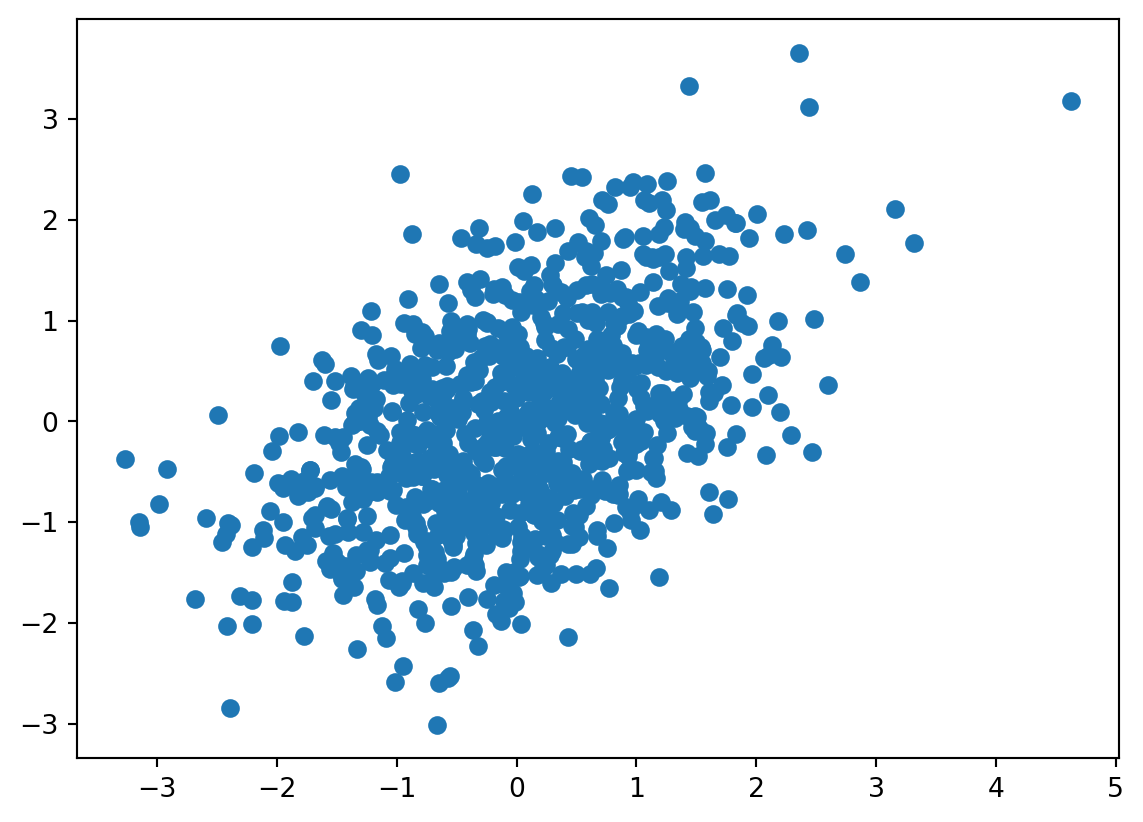

X = X - X.mean(0)
print(X.mean(0))
Sigma_hat = np.matmul(np.transpose(X), X) / (n-1) 
Sigma_hat

[-6.88338275e-18 -2.02060590e-17]

array([[1.07377785, 0.50162145],
       [0.50162145, 1.01008348]])

evd = la.eig(Sigma_hat)
lambda_ = evd[0]
v_hat = evd[1]
u_hat = np.matmul(X, np.transpose(v_hat))
plt.scatter(u_hat[:,0], u_hat[:,1])

<matplotlib.collections.PathCollection at 0x7d2d4f3b5810>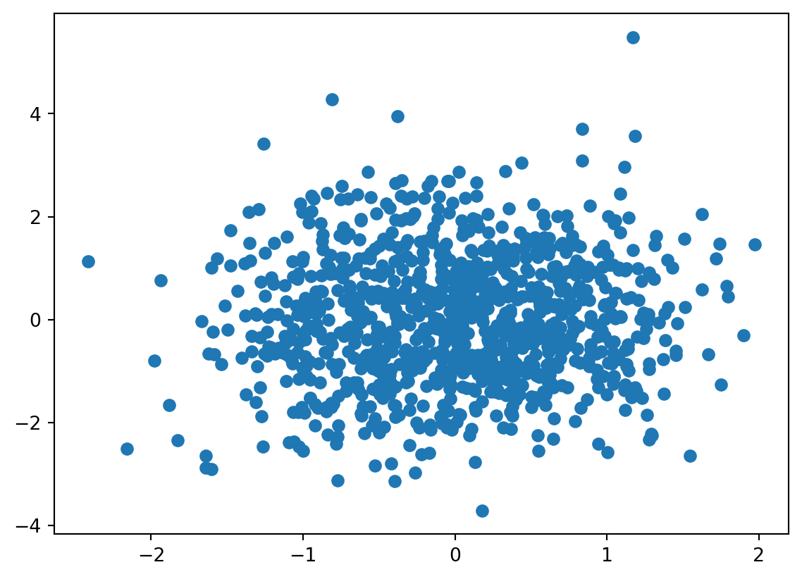

Fit using scikitlearn’s function

pca = PCA(n_components = 2).fit(X)
print(pca.explained_variance_)
print(lambda_ )

[1.54456206 0.53929927]
[1.54456206 0.53929927]

10.1.4 Example

Let’s consider the melanoma dataset that we looked at before. First we read in the data as we have done before so we don’t show that code.

Using downloaded and verified file: /home/bcaffo/.medmnist/dermamnist.npz
Using downloaded and verified file: /home/bcaffo/.medmnist/dermamnist.npz

Using downloaded and verified file: /home/bcaffo/.medmnist/dermamnist.npz

Next, let’s get the data from the torch dataloader format back into an image array and a matrix with the image part (28, 28, 3) vectorized.

def loader_to_array(dataloader):
  ## Read one iteration to get data
  test_input, test_target = iter(dataloader).next()
  ## Total number of training images
  n = np.sum([inputs.shape[0] for inputs, targets in dataloader])
  ## The dimensions of the images
  imgdim = (test_input.shape[2], test_input.shape[3])
  images = np.empty( (n, imgdim[0], imgdim[1], 3))

  ## Read the data from the data loader into our numpy array
  idx = 0
  for inputs, targets in dataloader:
    inputs = inputs.detach().numpy()
    for j in range(inputs.shape[0]):
      img = inputs[j,:,:,:]
      ## get it out of pytorch format
      img = np.transpose(img, (1, 2, 0))
      images[idx,:,:,:] = img
      idx += 1
  matrix = images.reshape(n, 3 * np.prod(imgdim))
  return images, matrix

train_images, train_matrix = loader_to_array(train_loader)
test_images, test_matrix = loader_to_array(test_loader)

## Demean the matrices
train_mean = train_matrix.mean(0)
train_matrix = train_matrix - train_mean
test_mean = test_matrix.mean(0)
test_matrix = test_matrix - test_mean

Now let’s actually perform PCA using scikitlearn. We’ll plot the eigenvalues divided by their sums, \(\lambda_k / \sum_{k'} \lambda_{k'}\). This is called a scree plot.

from sklearn.decomposition import PCA
n_comp = 10
pca = PCA(n_components = n_comp).fit(train_matrix)
plt.plot(pca.explained_variance_ratio_)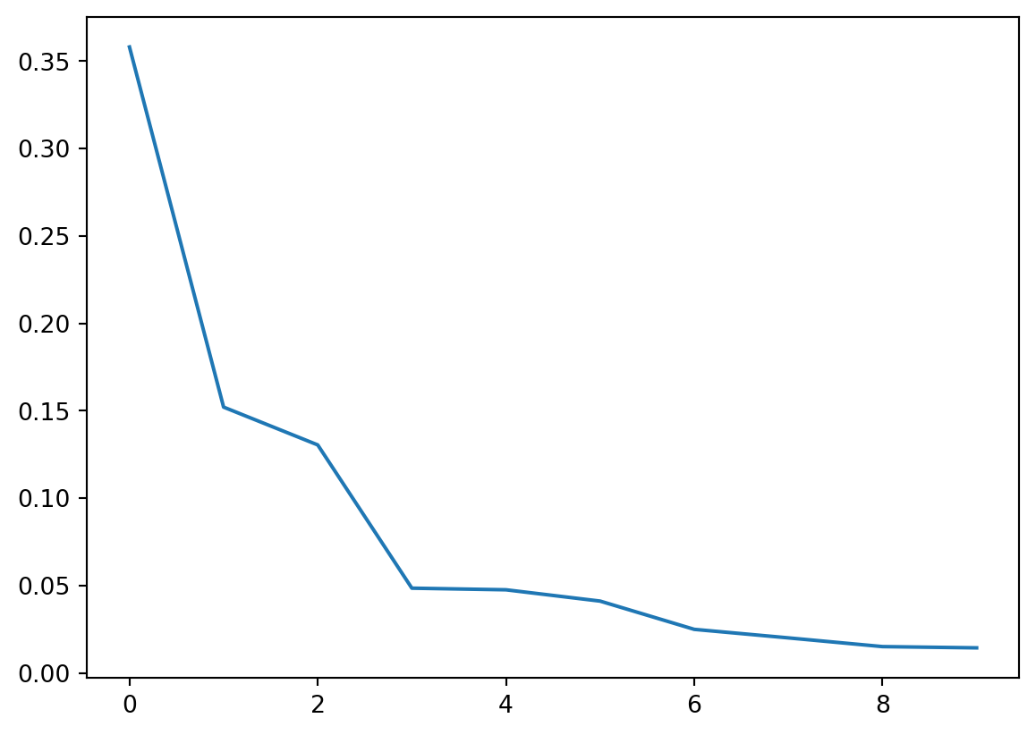

Often this is done by plotting the cummulative sum so that you can visualize how much variance is explained by including the top \(k\) components. Here I fit 10 components and they explain 85% of the variation.

plt.plot(np.cumsum(pca.explained_variance_ratio_))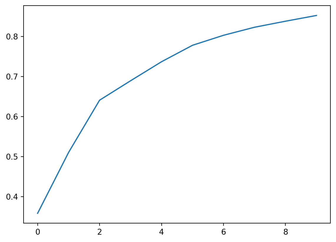

Note that the weights from the eigenvectors, \(V\), are images. We can plot these as images.

eigen_moles = pca.components_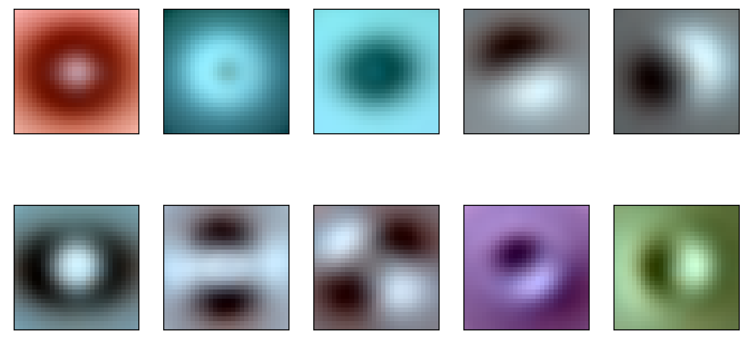

Let’s project our testing data onto the principal component basis created by our training data and see how it does. Let \(X_{training} = U \Lambda^{1/2} V^t\) is the SVD of our training data. Then, we can convert ths scores, \(U\) back to \(X_{training}\) with the map \(U \rightarrow U \lambda^{1/2} V\). Or, if our scores are normalized, \(U \Lambda^{1/2}\) then we simply multiply by \(V^t\). If we want to represent \(X_{training}\) by a lower dimensional summary, we just keep fewer columns of scores, then multiply by the same columns of \(V\). We could write this as \(U_s = X_{training} V_S \lambda^{-1/2}_S\), where \(S\) refers to a subset of values of \(k\).

Notice that \(\hat X_{training} = U_{S} V^t_S \Lambda^{-1/2}_S = X_{training} V_S V_S^t\) , \(\Lambda\) and \(V\). Consider then an approximation to \(X_{test}\) as \(\hat X_{test} = X_{test} V_s V_S^t\). Written otherwise \[ \hat X_{i,test} = \sum_{k \in S} <x_{i,test}, v_k> v_k \] which is the projection of subject \(i\)’s features into the linear space spanned by the basis defined by the principal component loadings.

Let’s try this on our mole data.

test_matrix_fit = pca.inverse_transform(pca.transform(test_matrix))
np.mean(np.abs( test_matrix - test_matrix_fit))

0.03792391028744076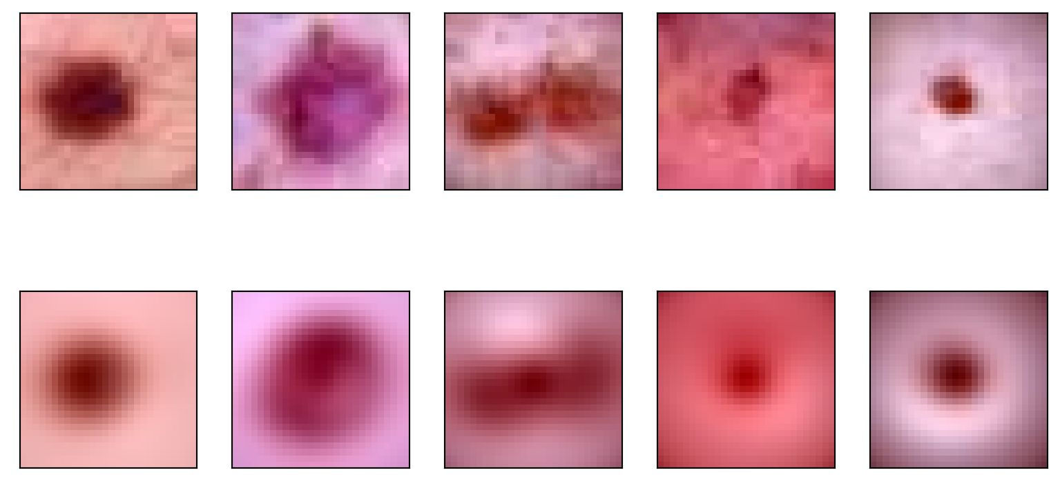

10.2 ICA

ICA, independent components analysis, tries to find linear transformations of the data that are statistically independent. Usually, independence is an assumption in ICA, not actually embedded in the loss function.

Let \(S_t\) be an \(\mathbb{R}^p\) collection of \(p\) source signals. Assume that the underlying signals are independent, so that \(S_t \sim F = F_1 \times F_2 \times \ldots \time f_p\). Assume that the observed data is \(X_t = M S_t\) and \(X_t \sim G\). It is typically assumed that \(M\) is invertible so that \(S_t = M^{-1} X_t\) and \(M\) and \(M^{-1}\) are called the mixing and unmixing matrices respectively. Note that, since we observe \(X_t\) over many repititions of \(t\), we can get an estimate of \(G\). Typically, it is also assumed that the \(X_t\) are iid over \(t\).

One way to characterize the estimation problem is to parameterize \(F_1\), \(F_2\) and \(F_3\) and use maximum likelihood, or equivalent [citations]. Another is to minimize some distance between \(G\) and \(F_1\), \(F_2\) and \(F_3\). Yet another is to actually maximize independence between the components of \(S_t\) using some estimate of independence [cite Matteson].

The most popular approaches try to find \(M^{-1}\) by maximizing non-Gaussianity. The logic goes that 1) interesting features tend to be non-Gaussian and 2) an appeal to the CLT over signals suggest that the mixed signals should be more Gaussian by being linear combinations of independent things. The latter claim is heuristic relative to the formal CLT. However, maximizing non-Gaussian components tends to work well in practice, thus validating the motivation empirically.

One form of ICA maximizes the kurtosis. If \(Y\) is a random variable, then \(E[Y^4] - 3 E[Y^2]\) is the kurtosis. One could then find \(M^{-1}\) that maximizes the empirical kurtosis of the unmixed signals. Another variation of non-Gaussianity maximizes neg-entropy. The neg-entropy of a density \(h\) is given by \[ - \int h(y) \log(h(y)) dy = - E_h[\log h(Y)] \] A well known theorem states that the Gaussian distribution has the largest entropy of all distributions with the same variance. Therefore, to maximize non-Gaussianity, we can minmize entropy, or equivalently maximize neg-entropy. We could subtract the entropy of the Gaussian distribution to consider this a cross entropy problem, but that only adds a constant to the loss function. The maximization of neg-entropy can be done many ways. We need the following. For a given \(M^{-1}\), estimate \(G\) from the collection \(M^{-1} X_t\), then calculate the neg-entropy of \(f_j\). Use that to then take an opimization step of \(M\) is the right direction. Some versions of estimation use a polynomial expansion of the \(f_j\), which then typically only requires higher order moments, like kurtosis. Fast ICA is a particular implmementation of maximizing neg-entropy.

Statistical versions of ICA don’t require \(M\) to be invertible. Moreover, error terms can be added in which case you can see the connection between ICA and factor analytic models. However, factor analysis models tend to assume Gaussianity.

10.2.1 Example

Consider an example that PCA would have somewhat of a hard time with. In this case, our data is from a mixture of normals with half from a normal with a strong positive correlation and half with a strong negative correlation. Because the angle between the two is not 90 degrees PCA has no chance. No rotation of the axes satisfies the obvious structure in this data.

n = 1000

Sigma = np.matrix([[4, 1.8], [1.8, 1]])
a = np.random.multivariate_normal( mean = [0, 0], cov = Sigma, size = int(n/2))
Sigma = np.matrix([[4, -1.8], [-1.8, 1]])
b = np.random.multivariate_normal( mean = [0, 0], cov = Sigma, size = int(n/2))
x = np.append( a, b, axis = 0)
plt.scatter(x[:,0], x[:,1])
plt.xlim([-6, 6])
plt.ylim([-6, 6])

(-6.0, 6.0)

Let’s try fast ICA. Notice it comes much closer to discovering the structure we’d like to discover than PCA could. It pulls appart the two components to a fair degree. Also note, there’s a random starting point of ICA, so that I get fairly different fits over re-runs of the algorithm. I had to lower the tolerance to get a good fit.

Indpendent components are order invariant and sign invariant.

transformer = FastICA(tol = 1e-7)
icafit = transformer.fit(x)
s = icafit.transform(x)
plt.scatter(s[:,0], s[:,1])
plt.xlim( [s.min(), s.max()])
plt.ylim( [s.min(), s.max()])

/home/bcaffo/miniconda3/envs/ds4bio/lib/python3.10/site-packages/sklearn/decomposition/_fastica.py:488: FutureWarning:

From version 1.3 whiten='unit-variance' will be used by default.

/home/bcaffo/miniconda3/envs/ds4bio/lib/python3.10/site-packages/sklearn/decomposition/_fastica.py:120: ConvergenceWarning:

FastICA did not converge. Consider increasing tolerance or the maximum number of iterations.

(-0.14345493269991716, 0.1408356388606491)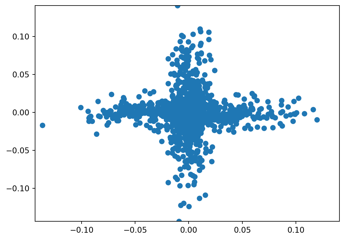

10.2.2 Cocktail party example

The classic ICA problem is the so called cocktail party problem. In this, you have \(p\) sources and \(p\) microphones. The microphones each pick up a mixture of signals from the different sources. The goal is to unmix the sources into the components. Independence makes sense in the cocktail party example, since logically conversations would have some independence.

import audio2numpy as a2n
s1, i1 = a2n.audio_from_file("mp3s/4.mp3")
s2, i2 = a2n.audio_from_file("mp3s/2.mp3")
s3, i3 = a2n.audio_from_file("mp3s/6.mp3")

## Get everything to be the same shape and sum the two audio channels
n = np.min((s1.shape[0], s2.shape[0], s3.shape[0]))
s1 = s1[0:n,:].mean(axis = 1)
s2 = s2[0:n,:].mean(axis = 1)
s3 = s3[0:n,:].mean(axis = 1)

s = np.matrix([s1, s2, s3])

Mix the signals.

w = np.matrix( [ [.7, .2, .1], [.1, .7, .2], [.2, .1, .7] ])
x = np.transpose(np.matmul(w, s))

Here’s an example mixed signal

IPython.display.Audio(data = x[:,1].reshape(n), rate = i1)

Now try to unmix using fastICA

transformer = FastICA(whiten=True, tol = 1e-7)
icafit = transformer.fit(x)

/home/bcaffo/miniconda3/envs/ds4bio/lib/python3.10/site-packages/sklearn/decomposition/_fastica.py:673: FutureWarning:

From version 1.3 whiten=True should be specified as whiten='arbitrary-variance' (its current behaviour). This behavior is deprecated in 1.1 and will raise ValueError in 1.3.

/home/bcaffo/miniconda3/envs/ds4bio/lib/python3.10/site-packages/sklearn/utils/validation.py:727: FutureWarning:

np.matrix usage is deprecated in 1.0 and will raise a TypeError in 1.2. Please convert to a numpy array with np.asarray. For more information see: https://numpy.org/doc/stable/reference/generated/numpy.matrix.html

icafit.mixing_

array([[-12.70609981, -51.16254236,  16.57481899],
       [-44.0705694 ,  -7.49682052,  31.47133465],
       [ -5.51913194, -14.14746356, 108.62751866]])

Unmixing matrix

icafit.components_

array([[ 0.00166493, -0.02401024,  0.00670215],
       [-0.02080964,  0.00581294,  0.0014911 ],
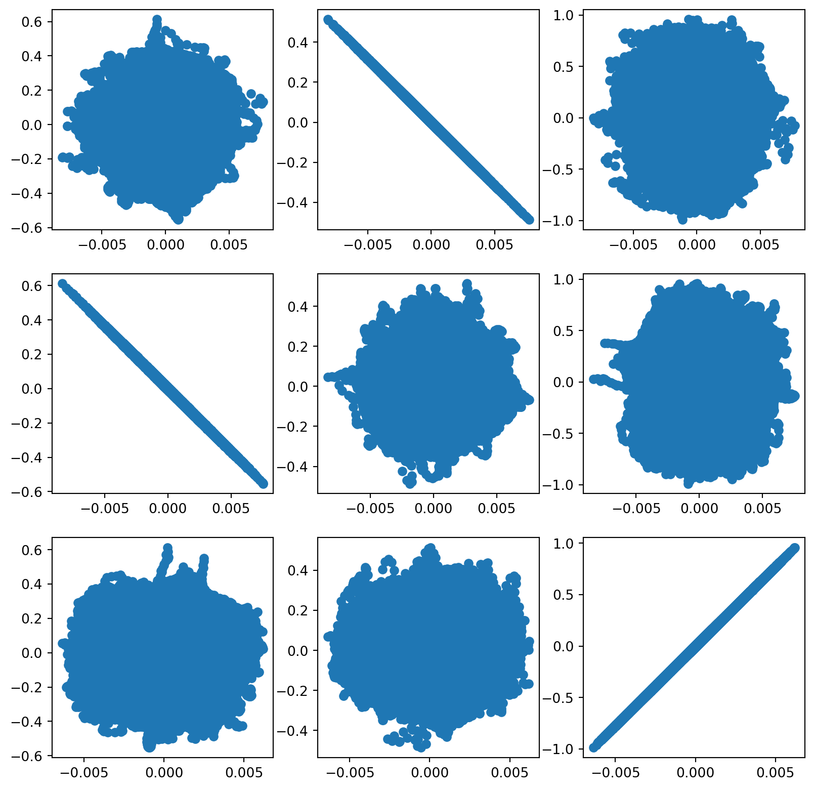
       [-0.00262562, -0.00046284,  0.00974049]])

Here’s a scatterplot matrix where the real component is on the rows and the estimated component is on the columns.

hat_s = np.transpose(icafit.transform(x))

plt.figure(figsize=(10,10))

for i in range(3):
  for j in range(3):
    plt.subplot(3, 3, (3 * i + j) + 1)
    plt.scatter(hat_s[i,:].squeeze(), np.asarray(s)[j,:])

/home/bcaffo/miniconda3/envs/ds4bio/lib/python3.10/site-packages/sklearn/utils/validation.py:727: FutureWarning:

np.matrix usage is deprecated in 1.0 and will raise a TypeError in 1.2. Please convert to a numpy array with np.asarray. For more information see: https://numpy.org/doc/stable/reference/generated/numpy.matrix.html

We can now play the estimated sources and see how they turned out.

from scipy.io.wavfile import write
i = 0
data = (hat_s[i,:].reshape(n) / np.max(np.abs(hat_s[i,:]))) * .5
IPython.display.Audio(data = data, rate = i1)

i = 1
data = (hat_s[i,:].reshape(n) / np.max(np.abs(hat_s[i,:]))) * .5
IPython.display.Audio(data = data, rate = i1)

i = 2
data = (hat_s[i,:].reshape(n) / np.max(np.abs(hat_s[i,:]))) * .5
IPython.display.Audio(data = data, rate = i1)

10.2.3 Imaging example using ICA

Let’s see what we get for the images. Logically, one would consider voxels as mixed sources and images as the iid replications. But, then the sources would not be images. Let’s try the other dimension and see what we get where subject images are mixtures of source images. This is analogous to finding a soure basis of subject images.

This is often done in ICA where people transpose matrices to investigate different problems.

transformer = FastICA(n_components=10, random_state=0,whiten='unit-variance', tol = 1e-7)
icafit = transformer.fit_transform(np.transpose(train_matrix))
icafit.shape

/home/bcaffo/miniconda3/envs/ds4bio/lib/python3.10/site-packages/sklearn/decomposition/_fastica.py:120: ConvergenceWarning:

FastICA did not converge. Consider increasing tolerance or the maximum number of iterations.

(2352, 10)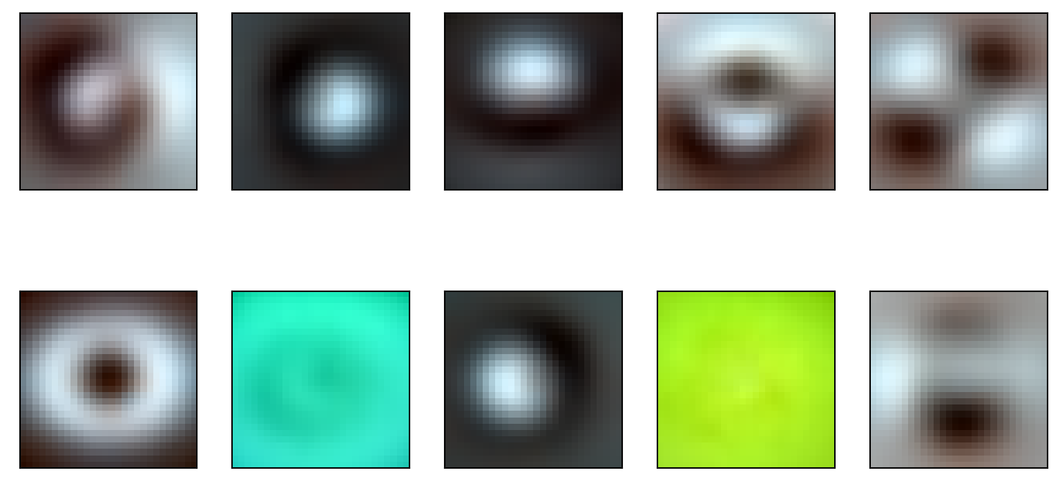

10.3 Autoencoders

Autoencoders are another unsupervised learning technique. Autoencoders take in a record and spit out a prediction of the same size. The goal is to represent the records as a NN. In an incomplete autoencoder, the model is regularized by the embedding (middle) layer being much lower than the input dimension. In this way, an autoencoder is a dimension reduction technique, reducing the input dimension size downto a much lower size (the encoder) then back out to the original size (the decoder). We can represent the autoencoder with a network diagram as below.

Let \(\phi\) be the first two layers of the network and \(\theta\) be the last two. So, if we wanted to pass a data row, \(x_i\) through the network we would do \(\theta(\phi(x_i))\). We would call the network \(\phi\) as the encoding network and \(\theta\) as the decoding network. Consider training the network by minimizing

\[ \sum_{i=1}^n || x_i - \theta(\phi(x_i)) ||^2 \]

over the weights. This sort of network is called an autoencoder. Notice that the same data is the input and output of the network. This kind of learning is called unsupervised, since we’re not trying to use \(x\) to predict an outcome \(y\). Instead, we’re trying to explore variation and find interesting features in \(x\) as a goal in itself without a “supervising” outcome, \(y\), to help out.

Notice overfitting concerns are somewhat different in this network construction. If this model fits well, then it’s suggesting that 2 numbers can explain 8. That is, the network will have reduced the inputs to only two dimensions, that we could visualize for example. That is a form of parsimony that prevents overfitting. The middle layer is called the embedding. It is called this because an autoencoder is a form of non-linear embedding of our data into a lower dimensionional space.

There’s nothing to prevent us from having convolutional layers if the inputs are images. That’s what we’ll work on here. For convolutional autoencoders, it’s typical to increase the number of channels and decrease the image sizes as one works through the network.

10.3.1 PCA and autoencoders

Without modification, autoencoders can be programmed that span the same space as PCA/SVD (Plaut 2018). Enforcing the orthogonality requires something like adding Lagrange terms to the loss function. There’s no reason why you would do this, since PCA is well developed and works just fine. However, it does suggest why NNs are such a large class of models.

Let \(X_i\) be a collection of features for record \(i\). Then, the SVD approximates the data matrix \(X\) with \(UV^t\), where we’ve absorbed the singular values into either \(U\) or \(V\). Per record, this model for \(K\) components and column \(k\) from \(V\) of \(v_k\).

\[ \hat x_i = \sum_{k=1}^K <x_i, v_k> v_k \]

Therefore, consider a neural network that specifies that the first layer defines \(K\) hidden units as

\[ h_{ik} = <x_i, v_k>. \]

That is, it has a linear activation function with no bias term and weights \(v_{jk}\) where \(v_{jk}\) is element \(j\) of vector \(v_k\). Then consider an output layer that defines

\[ \hat x_{ij} = \sum_{k=1}^K h_{ik} v_{jk}, \]

Again, this is a linear activation function with weights \(v_{jk}\). So, we arrive at the conclusion, that PCA is an example of an autoencoder with two layers, constraints on the weights being common to both layers, and constraints on the loss function that enforces the orthonormality of the \(v_k\). Of course, as we saw with ordinary regression, whether or not we can actually get gradient descent to converge remains a harder issue than just using PCA directly. Furthermore, the autoencoder wouldn’t necessarily order the PCs similarly.

Finally, we see that a two layer autoencoder -without the constraints- contains the PCA fit as a special case and spans the same space as the PCA fit. Similarly we see that such a two layer encoder is overspecified, as most NNs are.

10.3.2 Example on dermamnist

First, let’s set up our autoencoder by defining a python class then initializing it.

kernel_size = 5

class autoencoder(nn.Module):
    def __init__(self):
        super().__init__()
        
        self.conv1 = nn.Conv2d(3, 6, kernel_size)
        self.conv2 = nn.Conv2d(6, 12, kernel_size)
        self.pool  = nn.MaxPool2d(2, 2)
        self.iconv1 = nn.ConvTranspose2d(12, 6, kernel_size+1, stride = 2)
        self.iconv2 = nn.ConvTranspose2d(6, 3, kernel_size+1, stride = 2)

    def encode(self, x):
        x = F.relu(self.conv1(x))
        x = self.pool(x)
        x = F.relu(self.conv2(x))
        x = self.pool(x)
        return x
    
    def decode(self, x):
        x = F.relu(self.iconv1(x))
        ## Use the sigmoid as the final layer 
        ## since we've normalized pixel values to be between 0 and 1
        x = torch.sigmoid(self.iconv2(x))
        return(x)
    
    def forward(self, x):
        return self.decode(self.encode(x))
    
autoencoder = autoencoder()

We can try out the autoencoder by

## Here's some example data by grabbing one batch
tryItOut, _ = iter(train_loader).next()
print(tryItOut.shape)

## Let's encode that data
encoded = autoencoder.encode(tryItOut)
print(encoded.shape)

## Now let's decode the encoded data
decoded = autoencoder.decode(encoded)
print(decoded.shape)

## Now let's run the whole thing through
fedForward = autoencoder.forward(tryItOut)
print(fedForward.shape)

torch.Size([128, 3, 28, 28])
torch.Size([128, 12, 4, 4])
torch.Size([128, 3, 28, 28])
torch.Size([128, 3, 28, 28])

test = fedForward.detach().numpy()

## Plot out the first 5 images, note this isn't very interesting, since
## all of the weights haven't been trained
plt.figure(figsize=(10,5))
for i in range(5): 
  plt.subplot(1, 5,i+1)
  plt.xticks([])
  plt.yticks([])
  img = np.transpose(test[i,:,:,:], (1, 2, 0))
  plt.imshow(img)

#Optimizer
optimizer = torch.optim.Adam(autoencoder.parameters(), lr = 0.001)

#Epochs
n_epochs = 20

autoencoder.train()

for epoch in range(n_epochs):
    for data, _ in train_loader:
        images = data
        optimizer.zero_grad()
        outputs = autoencoder.forward(images)
        loss = F.mse_loss(outputs, images)
        loss.backward()
        optimizer.step()

## the data from the last iteration is called images
trainSample = images.detach().numpy()

plt.figure(figsize=(10,5))
for i in range(5): 
  plt.subplot(1, 5,i+1)
  plt.xticks([])
  plt.yticks([])
  img = np.transpose(trainSample[i,:,:,:], (1, 2, 0))
  plt.imshow(img)

## the output from the last iterations (feed forward through the network) is called outputs
trainOutput = outputs.detach().numpy()

plt.figure(figsize=(10,5))
for i in range(5): 
  plt.subplot(2, 5,i+6)
  plt.xticks([])
  plt.yticks([])
  img = np.transpose(trainOutput[i,:,:,:], (1, 2, 0))
  plt.imshow(img)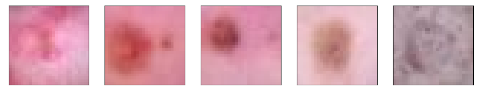

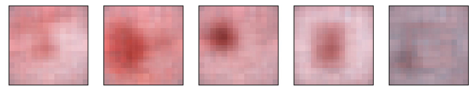
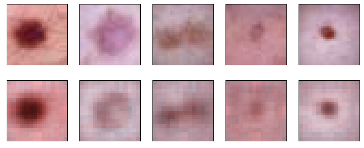
On a test batch

test_batch, _ = iter(test_loader).next()
x_test = test_batch.detach().numpy()
testSample = autoencoder.forward(test_batch).detach().numpy()

plt.figure(figsize=(10,4))

## Plot the original data
for i in range(5): 
  plt.subplot(2, 5, i + 1)
  plt.xticks([])
  plt.yticks([])
  img = np.transpose(x_test[i,:,:,:], (1, 2, 0))
  plt.imshow(img)
# Plot the data having been run throught the convolutional autoencoder
for i in range(5): 
  plt.subplot(2, 5, i + 6)
  plt.xticks([])
  plt.yticks([])
  img = np.transpose(testSample[i,:,:,:], (1, 2, 0))
  plt.imshow(img)

Plaut, Elad. 2018. “From Principal Subspaces to Principal Components with Linear Autoencoders.” arXiv Preprint arXiv:1804.10253.