Basic regression in pytorch

import pandas as pd
import torch
import statsmodels.formula.api as smf
import statsmodels as sm
import seaborn as sns
import matplotlib.pyplot as plt

## Read in the data and display a few rows
dat = pd.read_csv("https://raw.githubusercontent.com/bcaffo/ds4bme_intro/master/data/oasis.csv")
dat.head(4)

	FLAIR	PD	T1	T2	FLAIR_10	PD_10	T1_10	T2_10	FLAIR_20	PD_20	T1_20	T2_20	GOLD_Lesions
0	1.143692	1.586219	-0.799859	1.634467	0.437568	0.823800	-0.002059	0.573663	0.279832	0.548341	0.219136	0.298662	0
1	1.652552	1.766672	-1.250992	0.921230	0.663037	0.880250	-0.422060	0.542597	0.422182	0.549711	0.061573	0.280972	0
2	1.036099	0.262042	-0.858565	-0.058211	-0.044280	-0.308569	0.014766	-0.256075	-0.136532	-0.350905	0.020673	-0.259914	0
3	1.037692	0.011104	-1.228796	-0.470222	-0.013971	-0.000498	-0.395575	-0.221900	0.000807	-0.003085	-0.193249	-0.139284	0

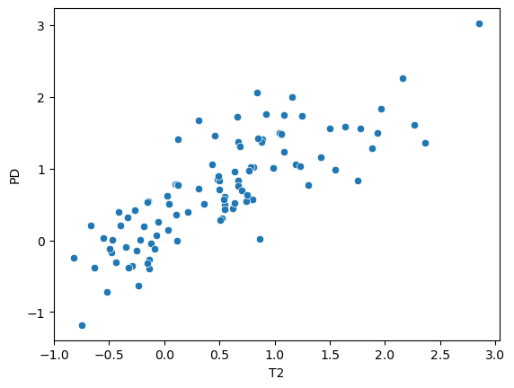
sns.scatterplot(x = dat['T2'], y = dat['PD'])

<Axes: xlabel='T2', ylabel='PD'>

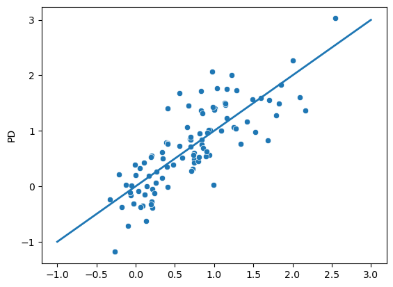
fit = smf.ols('PD ~ T2', data = dat).fit()
fit.summary()

OLS Regression Results

Dep. Variable:	PD	R-squared:	0.661
Model:	OLS	Adj. R-squared:	0.657
Method:	Least Squares	F-statistic:	190.9
Date:	Mon, 29 Jan 2024	Prob (F-statistic):	9.77e-25
Time:	07:02:58	Log-Likelihood:	-57.347
No. Observations:	100	AIC:	118.7
Df Residuals:	98	BIC:	123.9
Df Model:	1
Covariance Type:	nonrobust

	coef	std err	t	P>|t|	[0.025	0.975]
Intercept	0.3138	0.052	6.010	0.000	0.210	0.417
T2	0.7832	0.057	13.815	0.000	0.671	0.896

Omnibus:	1.171	Durbin-Watson:	1.501
Prob(Omnibus):	0.557	Jarque-Bera (JB):	0.972
Skew:	0.241	Prob(JB):	0.615
Kurtosis:	2.995	Cond. No.	1.89

Notes:
[1] Standard Errors assume that the covariance matrix of the errors is correctly specified.

# The in sample predictions
yhat = fit.predict(dat['T2'])

# Make sure that it's adding the intercept
#test = 0.3138 + dat['T2'] * 0.7832
#sns.scatterplot(yhat,test)

## A plot of the in sample predicted values
## versus the actual outcomes
sns.scatterplot(x = yhat, y = dat['PD'])
plt.plot([-1, 3], [-1, 3], linewidth=2)

[<matplotlib.lines.Line2D at 0x783ee16ecca0>]

n = dat.shape[0]

## Get the y and x from 
xtraining = torch.from_numpy(dat['T2'].values)
ytraining = torch.from_numpy(dat['PD'].values)

## PT wants floats
xtraining = xtraining.float()
ytraining = ytraining.float()

## Dimension is 1xn not nx1
## squeeze the second dimension
xtraining = xtraining.unsqueeze(1)
ytraining = ytraining.unsqueeze(1)

## Show that everything is the right size
[xtraining.shape, 
 ytraining.shape,
 [n, 1]
 ]

[torch.Size([100, 1]), torch.Size([100, 1]), [100, 1]]

## Show that linear regression is a pytorch 
model = torch.nn.Sequential(
    torch.nn.Linear(1, 1)
)

## MSE is the loss function
loss_fn = torch.nn.MSELoss(reduction='sum')

## Set the optimizer
## There are lots of choices
optimizer = torch.optim.SGD(model.parameters(), lr=1e-4)

## Loop over iterations
for t in range(10000):

    ## Forward propagation
  y_pred = model(xtraining)
    
  ## the loss for this interation
  loss = loss_fn(y_pred, ytraining)

  #print(t, loss.item() / n)

  ## Zero out the gradients before adding them up 
  optimizer.zero_grad()
  
  ## Backprop
  loss.backward()
  
  ## Optimization step
  optimizer.step()

ytest = model(xtraining).detach().numpy().reshape(-1)
sns.scatterplot(x = ytest, y = yhat)
plt.plot([-1, 3], [-1, 3], linewidth=2)

[<matplotlib.lines.Line2D at 0x783ee986a710>]

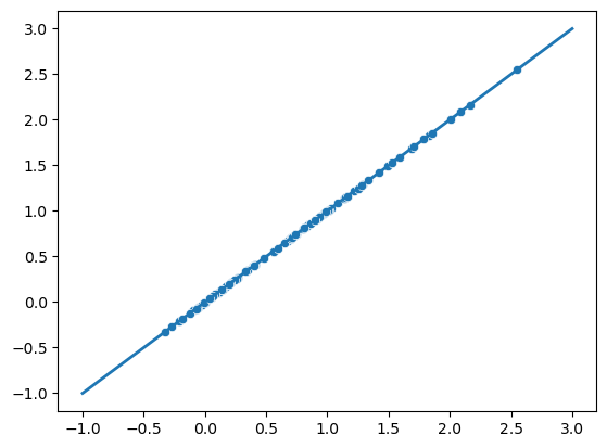
for param in model.parameters():
  print(param.data)

tensor([[0.7831]])
tensor([0.3138])