
![]()
Data cleaning by example#
We’re going to cover data cleaning by an example. Primarily, you’re going to work in pandas, a library for manipulating tabular data.
Imports and files#
The first thing we’ll try is loading some data and plotting it. To do this, we’ll need some packages. Let’s load up pandas, a package for data management, and matplotlib. The python command for this is import.
import pandas as pd ## Pandas is our main data cleaning library
import numpy as np ## Numpy is our main numerical library
import matplotlib as mpl ## Matplotlib is our main plotting library
Reading data in with pandas#
Let’s now read in an MRICloud dataset using pandas. We want to use the function read_csv within pandas. Notice we imported pandas as pd so the command is pd.read_csv. Also, pandas can accept URLs, so we just put the link to the file in the argument. The data we want to read in is in a github repo I created.
## Pandas can read in from a URL
df = pd.read_csv("https://raw.githubusercontent.com/bcaffo/ds4bme_intro/master/data/kirby127a_3_1_ax_283Labels_M2_corrected_stats.csv")
Let’s look at the first 4 rows of our dataframe. The object dataset is a pandas object with associated methods. One is head which allows one to see the first few rows of data.
df.head(4)
| Unnamed: 0 | rawid | roi | volume | min | max | mean | std | type | level | |
|---|---|---|---|---|---|---|---|---|---|---|
| 0 | 1 | kirby127a_3_1_ax.img | Telencephalon_L | 531111 | 0 | 374 | 128.3013 | 51.8593 | 1 | 1 |
| 1 | 2 | kirby127a_3_1_ax.img | Telencephalon_R | 543404 | 0 | 300 | 135.0683 | 53.6471 | 1 | 1 |
| 2 | 3 | kirby127a_3_1_ax.img | Diencephalon_L | 9683 | 15 | 295 | 193.5488 | 32.2733 | 1 | 1 |
| 3 | 4 | kirby127a_3_1_ax.img | Diencephalon_R | 9678 | 10 | 335 | 193.7051 | 32.7869 | 1 | 1 |
Working with the data#
Let’s get rid of the column rawid and the unnamed column since they’re kind of useless for today’s lecture. Also let’s work with only the volume.
df = df.drop(['Unnamed: 0', 'rawid', 'min', 'max', 'mean', 'std'], axis = 1)
Now let’s create a column called icv for intra-cranial volume. ICV is defined as the summ of the Type I Level 1 structures and cerebrospinal fluid. For the rest of this lecture, we’re just going to look at this type and level.
## Extract the Type 1 Level 1 data
t1l1 = df.loc[(df['type'] == 1) & (df['level'] == 1)].copy()
## Create a new column based on ICV
t1l1['icv'] = sum(t1l1['volume'])
t1l1
| roi | volume | type | level | icv | |
|---|---|---|---|---|---|
| 0 | Telencephalon_L | 531111 | 1 | 1 | 1378295 |
| 1 | Telencephalon_R | 543404 | 1 | 1 | 1378295 |
| 2 | Diencephalon_L | 9683 | 1 | 1 | 1378295 |
| 3 | Diencephalon_R | 9678 | 1 | 1 | 1378295 |
| 4 | Mesencephalon | 10268 | 1 | 1 | 1378295 |
| 5 | Metencephalon | 159402 | 1 | 1 | 1378295 |
| 6 | Myelencephalon | 4973 | 1 | 1 | 1378295 |
| 7 | CSF | 109776 | 1 | 1 | 1378295 |
One can access variables with methods, like df.type, or using brackets like df[‘type’]. I prefer the latter, since it can accomodate things like spaces, periods or other special characters in the varible name.
In addition to defining new varibles using brackets, one can use assign. The .copy() command is used because I want a new dataframe, not just referencing the slices of the other.
Now the TBV is defined as the sum of the volume for all rows except CSF.
t1l1 = t1l1.assign(tbv = sum(t1l1['volume'][(t1l1['roi'] != 'CSF')]))
t1l1
| roi | volume | type | level | icv | tbv | |
|---|---|---|---|---|---|---|
| 0 | Telencephalon_L | 531111 | 1 | 1 | 1378295 | 1268519 |
| 1 | Telencephalon_R | 543404 | 1 | 1 | 1378295 | 1268519 |
| 2 | Diencephalon_L | 9683 | 1 | 1 | 1378295 | 1268519 |
| 3 | Diencephalon_R | 9678 | 1 | 1 | 1378295 | 1268519 |
| 4 | Mesencephalon | 10268 | 1 | 1 | 1378295 | 1268519 |
| 5 | Metencephalon | 159402 | 1 | 1 | 1378295 | 1268519 |
| 6 | Myelencephalon | 4973 | 1 | 1 | 1378295 | 1268519 |
| 7 | CSF | 109776 | 1 | 1 | 1378295 | 1268519 |
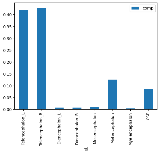
Let’s look at brain composition.
t1l1['comp'] = t1l1['volume'] / t1l1['tbv']
t1l1
| roi | volume | type | level | icv | tbv | comp | |
|---|---|---|---|---|---|---|---|
| 0 | Telencephalon_L | 531111 | 1 | 1 | 1378295 | 1268519 | 0.418686 |
| 1 | Telencephalon_R | 543404 | 1 | 1 | 1378295 | 1268519 | 0.428377 |
| 2 | Diencephalon_L | 9683 | 1 | 1 | 1378295 | 1268519 | 0.007633 |
| 3 | Diencephalon_R | 9678 | 1 | 1 | 1378295 | 1268519 | 0.007629 |
| 4 | Mesencephalon | 10268 | 1 | 1 | 1378295 | 1268519 | 0.008094 |
| 5 | Metencephalon | 159402 | 1 | 1 | 1378295 | 1268519 | 0.125660 |
| 6 | Myelencephalon | 4973 | 1 | 1 | 1378295 | 1268519 | 0.003920 |
| 7 | CSF | 109776 | 1 | 1 | 1378295 | 1268519 | 0.086539 |
Plotting#
Pandas has built in methods for plotting. Later on, we’ll try different plotting packages.
t1l1.plot.bar(x='roi',y='comp');
In colab, you have to install packages it doesn’t have everytime you reconnect the runtime. I’ve commented this out here, since plotly is already installed locally for me. To install in colab, use a ! in front of the unix command. In this case we’re using the python package management system pip to install plotly, an interactive graphing envinronment.
#!pip install plotly
We can create an interactive plot with plotly. This is a professionally developed package that makes interactive plotting very easy. Also, it renders nicely within colab or jupyter notebooks. For plotly graphics, I would suggest assigning the graph to a variable then calling that variable to show the plot. This way you can modify the plot later if you’d like.
import plotly.express as px
myplot = px.bar(t1l1, x='roi', y='volume')
myplot.show()