Logistic regression in pytorch

This is an extension of using pytorch to perform linear regression to using it to perform logistic regression.

import pandas as pd
import torch
import statsmodels.formula.api as smf
import statsmodels as sm
import seaborn as sns
import matplotlib.pyplot as plt
import numpy as np

## Read in the data and display a few rows
dat = pd.read_csv("https://raw.githubusercontent.com/bcaffo/ds4bme_intro/master/data/oasis.csv")
dat.head(4)

## Create a binary outcome variable (people will use gold lesions in HW)
m = np.median(dat.T2)
dat = dat.assign(y = (dat.T2 > m) * 1 )
## Create a normalized regression variable
dat = dat.assign(x = (dat.PD - np.mean(dat.PD)) / np.std(dat.PD))
dat.head()

	FLAIR	PD	T1	T2	FLAIR_10	PD_10	T1_10	T2_10	FLAIR_20	PD_20	T1_20	T2_20	GOLD_Lesions	y	x
0	1.143692	1.586219	-0.799859	1.634467	0.437568	0.823800	-0.002059	0.573663	0.279832	0.548341	0.219136	0.298662	0	1	1.181648
1	1.652552	1.766672	-1.250992	0.921230	0.663037	0.880250	-0.422060	0.542597	0.422182	0.549711	0.061573	0.280972	0	1	1.426453
2	1.036099	0.262042	-0.858565	-0.058211	-0.044280	-0.308569	0.014766	-0.256075	-0.136532	-0.350905	0.020673	-0.259914	0	0	-0.614749
3	1.037692	0.011104	-1.228796	-0.470222	-0.013971	-0.000498	-0.395575	-0.221900	0.000807	-0.003085	-0.193249	-0.139284	0	0	-0.955175
4	1.580589	1.730152	-0.860949	1.245609	0.617957	0.866352	-0.099919	0.384261	0.391133	0.608826	0.071648	0.340601	0	1	1.376909

fit = smf.logit('y ~ x', data = dat).fit()
fit.summary()

Optimization terminated successfully.
         Current function value: 0.427855
         Iterations 7

Logit Regression Results

Dep. Variable:	y	No. Observations:	100
Model:	Logit	Df Residuals:	98
Method:	MLE	Df Model:	1
Date:	Mon, 29 Jan 2024	Pseudo R-squ.:	0.3827
Time:	07:03:46	Log-Likelihood:	-42.785
converged:	True	LL-Null:	-69.315
Covariance Type:	nonrobust	LLR p-value:	3.238e-13

	coef	std err	z	P>|z|	[0.025	0.975]
Intercept	0.0367	0.269	0.136	0.892	-0.491	0.565
x	2.2226	0.436	5.095	0.000	1.368	3.078

# The in sample predictions
yhat = 1 / (1 + np.exp(-fit.fittedvalues))

n = dat.shape[0]

## Get the y and x from 
xtraining = torch.from_numpy(dat['x'].values)
ytraining = torch.from_numpy(dat['y'].values)

## PT wants floats
xtraining = xtraining.float()
ytraining = ytraining.float()

## Dimension is 1xn not nx1
## squeeze the second dimension
xtraining = xtraining.unsqueeze(1)
ytraining = ytraining.unsqueeze(1)

## Show that everything is the right size
[xtraining.shape, 
 ytraining.shape,
 [n, 1]
 ]

[torch.Size([100, 1]), torch.Size([100, 1]), [100, 1]]

## Doing it more now the pytorch docs recommend
## Example taken from 
## https://medium.com/biaslyai/pytorch-linear-and-logistic-regression-models-5c5f0da2cb9

## They recommend creating a class that defines
## the model
class LogisticRegression(torch.nn.Module):
     def __init__(self):
        super(LogisticRegression, self).__init__()
        self.linear = torch.nn.Linear(1, 1, bias = True)
     def forward(self, x):
        y_pred = torch.sigmoid(self.linear(x))
        return y_pred

## Then the model is simply  
model = LogisticRegression()

## MSE is the loss function
loss_fn = torch.nn.BCELoss()  

## Set the optimizer
optimizer = torch.optim.Adam(model.parameters(), lr=1e-4)

## Loop over iterations
for t in range(100000):

  ## Forward propagation
  y_pred = model(xtraining)

  ## the loss for this interation
  loss = loss_fn(y_pred, ytraining)

  #print(t, loss.item() / n)

  ## Zero out the gradients before adding them up 
  optimizer.zero_grad()
  
  ## Backprop
  loss.backward()
  
  ## Optimization step
  optimizer.step()

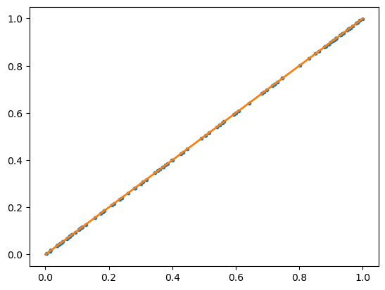
ytest = model(xtraining)
ytest = ytest.detach().numpy().reshape(-1)
plt.plot(yhat, ytest,  ".")
plt.plot([0, 1], [0, 1], linewidth=2)

[<matplotlib.lines.Line2D at 0x7b7316c8e680>]

for param in model.parameters():  
  print(param.data)

tensor([[1.4062]])
tensor([-0.0502])