
![]()
Linear separable models#
We’ve now covered two ways to do prediction with a single variable, classification using logistic regression and prediction using a line and least squares. What if we have several predictiors?
In both the logistic and linear regression models, we had a linear predictor, specifically,
In the continuous case, we were modeling the expected value of the outcomes as linear. In the binary case, we were assuming that the naturual logarithm of the odds of a 1 outcome was linear.
To estimate the unknown parameters, \(\beta_0\) and \(\beta_1\) we minimized
in the linear case and
in the binary outcome case (where, recall, \(\eta_i\) depends on the parameters). We can easily extend these models to multiple predictors by assuming that the impact of the multiple predictors is linear and separable. That is,
If we think about this as vectors and matrices, we obtain
where \(\eta\) is an \(n \times 1\) vector, \(X\) is an \(n \times p\) matrix with \(i,j\) entry \(x_{ij}\) and \(\beta\) is a \(p\times 1\) vector with entries \(\beta_j\).
Let’s look at the voxel-level data that we’ve been working with. First let’s load the data.
import numpy as np
import pandas as pd
import seaborn as sns
import matplotlib.pyplot as plt
import sklearn.linear_model as lm
import sklearn as skl
import statsmodels.formula.api as smf
import statsmodels as sm

## this sets some style parameters
sns.set()

## Read in the data
dat = pd.read_csv("https://raw.githubusercontent.com/bcaffo/ds4bme_intro/master/data/oasis.csv")
Let’s first try to fit the proton density data from the other imaging data. I’m going to use the statsmodels version of linear models since it has a nice format for dataframes.
trainFraction = .75

sample = np.random.uniform(size = 100) < trainFraction
trainingDat = dat[sample]
testingDat = dat[~sample]
results = smf.ols('PD ~ FLAIR + T1 + T2  + FLAIR_10 + T1_10 + T2_10 + FLAIR_20', data = trainingDat).fit()
print(results.summary2())
                 Results: Ordinary least squares
=================================================================
Model:              OLS              Adj. R-squared:     0.780
Dependent Variable: PD               AIC:                65.4823
Date:               2024-01-29 06:47 BIC:                84.0222
No. Observations:   75               Log-Likelihood:     -24.741
Df Model:           7                F-statistic:        38.48
Df Residuals:       67               Prob (F-statistic): 4.34e-21
R-squared:          0.801            Scale:              0.12678
------------------------------------------------------------------
               Coef.   Std.Err.     t     P>|t|    [0.025   0.975]
------------------------------------------------------------------
Intercept      0.1001    0.1278   0.7832  0.4362  -0.1549   0.3551
FLAIR          0.0537    0.0774   0.6934  0.4905  -0.1008   0.2081
T1            -0.3114    0.0842  -3.6993  0.0004  -0.4794  -0.1434
T2             0.5366    0.0830   6.4681  0.0000   0.3710   0.7022
FLAIR_10       0.0698    0.3321   0.2102  0.8341  -0.5931   0.7327
T1_10          0.3136    0.1531   2.0480  0.0445   0.0080   0.6193
T2_10          0.2117    0.2849   0.7431  0.4600  -0.3569   0.7803
FLAIR_20       1.2552    0.7459   1.6827  0.0971  -0.2337   2.7441
-----------------------------------------------------------------
Omnibus:              1.233        Durbin-Watson:           1.844
Prob(Omnibus):        0.540        Jarque-Bera (JB):        0.763
Skew:                 0.230        Prob(JB):                0.683
Kurtosis:             3.179        Condition No.:           42
=================================================================
Notes:
[1] Standard Errors assume that the covariance matrix of the
errors is correctly specified.
x = dat[['FLAIR','T1', 'T2', 'FLAIR_10', 'T1_10', 'T2_10', 'FLAIR_20']]
y = dat[['GOLD_Lesions']]
## Add the intercept column
x = sm.tools.add_constant(x)

xtraining = x[sample]
xtesting = x[~sample]
ytraining = y[sample]
ytesting = y[~sample]
fit = sm.discrete.discrete_model.Logit(ytraining, xtraining).fit()
Optimization terminated successfully.
         Current function value: 0.264729
         Iterations 8
print(fit.summary())
                           Logit Regression Results
==============================================================================
Dep. Variable:           GOLD_Lesions   No. Observations:                   75
Model:                          Logit   Df Residuals:                       67
Method:                           MLE   Df Model:                            7
Date:                Mon, 29 Jan 2024   Pseudo R-squ.:                  0.6176
Time:                        06:47:16   Log-Likelihood:                -19.855
converged:                       True   LL-Null:                       -51.926
Covariance Type:            nonrobust   LLR p-value:                 2.236e-11
==============================================================================
                 coef    std err          z      P>|z|      [0.025      0.975]
------------------------------------------------------------------------------
const         -4.8293      1.876     -2.574      0.010      -8.507      -1.152
FLAIR          2.2957      1.166      1.969      0.049       0.011       4.580
T1             2.3580      1.055      2.236      0.025       0.291       4.425
T2             2.1419      1.084      1.976      0.048       0.017       4.267
FLAIR_10       7.7567      3.677      2.109      0.035       0.550      14.964
T1_10          1.2147      1.572      0.773      0.440      -1.866       4.296
T2_10         -4.9682      3.051     -1.628      0.103     -10.949       1.012
FLAIR_20     -18.1028      7.771     -2.330      0.020     -33.334      -2.872
==============================================================================
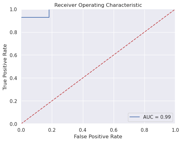
Now let’s evaluate our prediction. Here, we’re not going to classify as 0 or 1, but rather estimate the prediction. Note, we then would need to pick a threshold to have a classifier. We could use .5 as our threshold. However, it’s often the case that we don’t necessarily want to threshold at specifically that level. A solution for evalution is to plot how the sensitivity and specificity change by the threshold.
In other words, consider the triplets
$\(
(t, sens(t), spec(t))
\)\(
where \)t\( is the threshold, `sens(t)` is the sensitivity at threshold \)t$, spec(t) is the specificity at threshold t.
Necessarily, the sensitivity and specificity
phatTesting = fit.predict(xtesting)

## See here for plotting
## https://stackoverflow.com/questions/25009284/how-to-plot-roc-curve-in-python
fpr, tpr, threshold = skl.metrics.roc_curve(ytesting, phatTesting)
roc_auc = skl.metrics.auc(fpr, tpr)

# method I: plt
import matplotlib.pyplot as plt
plt.title('Receiver Operating Characteristic')
plt.plot(fpr, tpr, 'b', label = 'AUC = %0.2f' % roc_auc)
plt.legend(loc = 'lower right')
plt.plot([0, 1], [0, 1],'r--')
plt.xlim([0, 1])
plt.ylim([0, 1])
plt.ylabel('True Positive Rate')
plt.xlabel('False Positive Rate')
plt.show()
Aside different python packages#
So far we’ve explored several plotting libraries including: default pandas methods, matplotlib, seaborn and plotly. We’ve also looked at several fitting libraries including to some extent numpy, but especially scikitlearn and statsmodels. What’s the difference? Well, these packages are all mantained by different people and have different features and goals. For example, scikitlearn is more expansive than statsmodels, but statsmodels functions more like one is used to with statistical output. Matplotlib is very expansive, but seaborn has nicer default options and is a little easier. So, when doing data science with python, one has to get used to trying out a few packages, weighing the cost and benefits of each, and picking one.
‘statsmodels’, what we’re using above, has multiple methods for fitting binary models including: sm.Logit, smf.logit, BinaryModel and glm. Here I’m just going to use Logit which does not use the formula syntax of logit. Note, by default, this does not add an intercept this way. So, I’m adding a column of ones, which adds an intercept.
Consider the following which uses the formula API
results = smf.logit(formula = 'GOLD_Lesions ~ FLAIR + T1 + T2 + FLAIR_10 + T1_10 + T2_10 + FLAIR_20', data = trainingDat).fit()
print(results.summary())
Optimization terminated successfully.
         Current function value: 0.264729
         Iterations 8
                           Logit Regression Results
==============================================================================
Dep. Variable:           GOLD_Lesions   No. Observations:                   75
Model:                          Logit   Df Residuals:                       67
Method:                           MLE   Df Model:                            7
Date:                Mon, 29 Jan 2024   Pseudo R-squ.:                  0.6176
Time:                        06:47:16   Log-Likelihood:                -19.855
converged:                       True   LL-Null:                       -51.926
Covariance Type:            nonrobust   LLR p-value:                 2.236e-11
==============================================================================
                 coef    std err          z      P>|z|      [0.025      0.975]
------------------------------------------------------------------------------
Intercept     -4.8293      1.876     -2.574      0.010      -8.507      -1.152
FLAIR          2.2957      1.166      1.969      0.049       0.011       4.580
T1             2.3580      1.055      2.236      0.025       0.291       4.425
T2             2.1419      1.084      1.976      0.048       0.017       4.267
FLAIR_10       7.7567      3.677      2.109      0.035       0.550      14.964
T1_10          1.2147      1.572      0.773      0.440      -1.866       4.296
T2_10         -4.9682      3.051     -1.628      0.103     -10.949       1.012
FLAIR_20     -18.1028      7.771     -2.330      0.020     -33.334      -2.872
==============================================================================