Regression through the origin

In this notebook, we investigate a simple poblem where we’d like to use one scaled regressor to predict another. That is, let $Y_1, \ldots Y_n$ be a collection of variables we’d like to predict and $X_1, \ldots, X_n$ be predictors. Consider minimizing

$$ l = \sum_i ( Y_i - \beta X_i)^2 = || Y - \beta X||^2. $$

Taking a derivative of $l$ with respect to $\beta$ yields

$$ l’ = - \sum_i 2 (Y_i - \beta X_i) X_i. $$

If we set this equal to zero and solve for beta we obtain the classic solution:

$$ \hat \beta = \frac{\sum_i Y_i X_i}{\sum_i X_i^2} = \frac{<Y, X>}{||X||^2}. $$

Note further, if we take a second derivative we get

$$ l’’ = \sum_i 2 x_i^2
$$

which is strictly positive unless all of the $x_i$ are zero (a case of zero variation in the predictor where regresssion is uninteresting). Regression through the origin is a very useful version of regression, but it’s quite limited in its application. Rarely do we want to fit a line that is forced to go through the origin, or stated equivalently, rarely do we want a prediction algorithm for $Y$ that is simply a scale change of $X$. Typically, we at least also want an intercept. In the example that follows, we’ll address this by centering the data so that the origin is the mean of the $Y$ and the mean of the $X$. As it turns out, this is the same as fitting the intercept, but we’ll do that more formally in the next section.

First let’s load the necessary packages.

import pandas as pd
import numpy as np
import matplotlib.pyplot as plt

Now let’s download and read in the data.

dat = pd.read_csv("https://raw.githubusercontent.com/bcaffo/ds4bme_intro/master/data/oasis.csv")
dat.head()

	FLAIR	PD	T1	T2	FLAIR_10	PD_10	T1_10	T2_10	FLAIR_20	PD_20	T1_20	T2_20	GOLD_Lesions
0	1.143692	1.586219	-0.799859	1.634467	0.437568	0.823800	-0.002059	0.573663	0.279832	0.548341	0.219136	0.298662	0
1	1.652552	1.766672	-1.250992	0.921230	0.663037	0.880250	-0.422060	0.542597	0.422182	0.549711	0.061573	0.280972	0
2	1.036099	0.262042	-0.858565	-0.058211	-0.044280	-0.308569	0.014766	-0.256075	-0.136532	-0.350905	0.020673	-0.259914	0
3	1.037692	0.011104	-1.228796	-0.470222	-0.013971	-0.000498	-0.395575	-0.221900	0.000807	-0.003085	-0.193249	-0.139284	0
4	1.580589	1.730152	-0.860949	1.245609	0.617957	0.866352	-0.099919	0.384261	0.391133	0.608826	0.071648	0.340601	0

It’s almost always a good idea to plot the data before fitting the model.

x = dat.T2
y = dat.PD
plt.plot(x, y, 'o')

[<matplotlib.lines.Line2D at 0x7d0538dd80a0>]

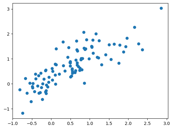
Now, let’s center the data as we mentioned so that it seems more reasonable to have the line go through the origin. Notice here, the middle of the data, both $Y$ and $X$, is right at (0, 0).

x = x - np.mean(x)
y = y - np.mean(y)
plt.plot(x, y, 'o')

[<matplotlib.lines.Line2D at 0x7d0538c606a0>]

Here’s our slope estimate according to our formula.

b = sum(y * x) / sum(x ** 2 )
b

0.7831514763655999

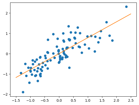
Let’s plot it so to see how it did. It looks good. Now let’s see if we can do a line that doesn’t necessarily have to go through the origin.

plt.plot(x, y, 'o')
t = np.array([-1.5, 2.5])
plt.plot(t, t * b)

[<matplotlib.lines.Line2D at 0x7d0530ac2e30>]