Unsupervised learning

Unsupervised learning#

PCA#

Let ${X_{i}}$ for $i = 1, \dots, n$ be $p$ random vectors with means $(0, \dots, 0)^{t}$ and variance matrix $Σ$ . Consider finding $v_{1}$ , a $p$ dimensional vector with $| | v_{1} | | = 1$ so that $v_{1}^{t} Σ v_{1}$ is maximized. Notice this is equivalent to saying we want to maximize $Var (X_{i}^{t} V_{1})$ . The well known solution to this equation is that $v_{1}$ is the first eigenvector of $Σ$ and $λ_{1} = Var (X_{i}^{t} V_{1})$ is the associated eigenvalue. If $Σ = V^{t} Λ V$ is the eigenvalue decomposition of where $V$ are the eigenvectors and $Λ$ is a diagonal matrix of the eigenvalues ordered from greatest to least, then $v_{1}$ corresponds to the first column of $V$ and $λ_{1}$ corresponds to the first element of $Λ$ . If one then finds $v_{k}$ as the vector maximizing $v_{k}^{t} Σ v_{k}$ so that $v_{k}^{t} v_{k^{'}} = I (k = k^{'})$ , then the $v_{k}$ are the columns of $V$ and $v_{k}^{t} Σ v_{k} = λ_{k}$ are the eigenvalues.

Notice:

$V Σ V^{t} = Λ$ (i.e. $V$ diagonalizess $Σ$ )
$Trace (Σ) = Trace (Σ V^{t} V) = Trace (V Σ V^{t}) = \sum λ_{k}$ (i.e. the total variability is the sum of the eigenvalues)
Since $V^{t} V = I$ , $V$ is a rotation matrix. Thus, $V$ rotates $X_{i}$ in such a way that to maximize variability in the first dimension, then the second dimensions …
$Cov (X_{i}^{t} v_{k}, x_{i}^{t} v_{k^{'}}) = Cov (X_{i}^{t} v_{k}, x_{i}^{t} v_{k^{'}}) v_{k}^{t} Cov (x_{i}, x_{i}^{t}) v_{k^{'}} = v_{k}^{t} V v_{k^{'}} = 0$ if $k \neq k^{'}$
Another representation of $Σ$ is $\sum_{k = 1}^{p} λ_{i} v_{k} v_{k}^{t}$ by simply rewriting the matrix algebra of $V Λ V^{t}$ .
The variables $U_{i} = V X_{i}$ then: have uncorrelated elements ( $Cov (U_{i k}, U_{i k^{'}}) = 0$ for $k \neq k^{'}$ by property 5), have the same total variability as the elements of $X_{i}$ ( $\sum_{k} Var (U_{i k}) = \sum_{k} λ_{k} = \sum_{k} Var (X_{i k})$ by property 2), are a rotation of the $X_{i}$ , are ordered so that $U_{i 1}$ has the greatest amount of variability and so on.

Notation:

The $λ_{k}$ are simply called the eigenvalues or principal components variation.
$U_{i k} = X_{i}^{t} v_{k}$ is called the principal component scores.
The $v_{k}$ are called the principal component loadings or weights, with $v_{1}$ being called the first principal component and so on.

Statistical properties under the assumption that the $x_{i}$ are iid with mean 0 and variance $Σ$

$E [U_{i k}] = 0$
$Var (U_{i k}) = λ_{k}$
$Cov (U_{i k}, U_{i k^{'}}) = 0$ if $k \neq k^{'}$
$\sum_{k = 1}^{p} Var (U_{i k}) = Trace (Σ)$ .
$\prod_{k = 1}^{p} Var (U_{i k}) = Det (Σ)$

Sample PCA#

Of course, we’re describing PCA as a conceptual process. We realize $n$ $p$ dimensional vectors $x_{1}$ to $x_{n}$ , typically organized in $X$ a $n \times p$ matrix. If $X$ is not mean 0, we typically demean it by calculating $(I - J (J^{t} J)^{- 1} J^{'}) X$ where $J$ is a vector of ones. Assume this is done. Then $\frac{1}{n - 1} X^{t} X = \hat{Σ}$ . Thus, our sample PCA is obtained via the eigenvalue decomposition $\hat{Σ} = \hat{V} \hat{Λ} {\hat{V}}^{t}$ and our principal components obtained as $X V$ .

We can relate PCA to the SVD as follows. Let $\frac{1}{\sqrt{n - 1}} X = \hat{U} {\hat{Λ}}^{1 / 2} {\hat{V}}^{t}$ be the SVD of the scaled version of $X$ . Then note that $ $\hat{Σ} = \frac{1}{n - 1} X^{t} X = \hat{V} \hat{Λ} {\hat{V}}^{t}$ $ yields the sample covariance matrix eigenvalue decomposition.

PCA with a large dimension#

Consider the case where one of $n$ or $p$ is large. Let’s assume $n$ is large. Then $ $\frac{1}{n - 1} X^{t} X = \frac{1}{n - 1} \sum_{i} x_{i} x_{i}^{t}$ $A s w e l e a r n e d i n t h e c h a p t e r o n H D F 5, w e c a n d o s u m s l i k e t h e s e w i t h o u t l o a d i n g t h e e n t i r e t y o f$ X $i n t o m e m o r y . T h u s, i n t h i s c a s e, w e c a n c a l c u l a t e t h e e i g e n v e c t o r s u s i n g o n l y t h e s m a l l d i m e n s i o n . I f, o n t h e o t h e r h a n d,$ p $i s l a r g e a n d$ n $i s s m a l l e r, t h e n w e c a n c a l c u l a t e t h e e i g e n v a l u e d e c o m p o s i t i o n o f$ $\frac{1}{n - 1} X X^{t} = \hat{U} \hat{Λ} {\hat{U}}^{t} .$ $I n e i t h e r c a s e, w h e t h e r$ U $o r$ V$ is easier to get, we can then obtain the other via vectorized multiplication.

Simple example#

## If you need to install the dependencies that aren't normally part of colab
#!pip install audio2numpy &> /dev/null
#!pip install medmnist &> /dev/null

import numpy as np
import matplotlib.pyplot as plt
import numpy.linalg as la
from sklearn.decomposition import PCA
import urllib.request
import PIL
import numpy as np
import torch
import torch.nn as nn
import torch.optim as optim
import torch.nn.functional as F
import torchvision
import torchvision.transforms as transforms
import torch.utils.data as data
from torch.utils.data import TensorDataset, DataLoader
from sklearn.decomposition import FastICA
from tqdm import tqdm
import medmnist
from medmnist import INFO, Evaluator
import scipy
import IPython
import audio2numpy as a2n

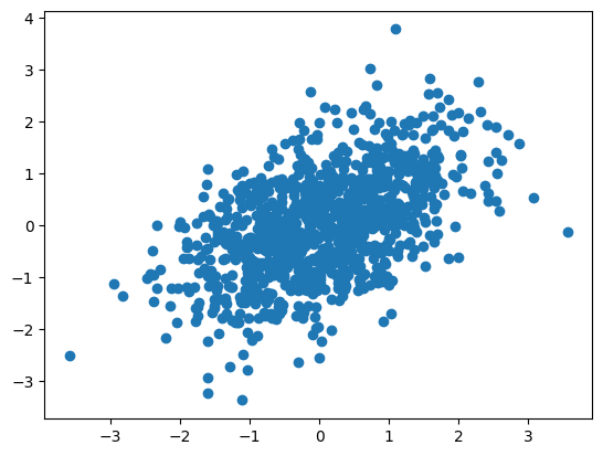
n = 1000
mu = (0, 0)
Sigma = np.array([[1, .5], [.5, 1]])
X = np.random.multivariate_normal( mean = mu, cov = Sigma, size = n)

plt.scatter(X[:,0], X[:,1]);

_images/9a8543fdd6901af060bd648bd31c7c59f80cb5acf79e85aad323966bf8b418d2.png

X = X - X.mean(0)
print(X.mean(0))
Sigma_hat = np.matmul(np.transpose(X), X) / (n-1)
Sigma_hat

[7.32747196e-18 3.84137167e-17]

array([[1.02255046, 0.52537753],
       [0.52537753, 0.99663657]])

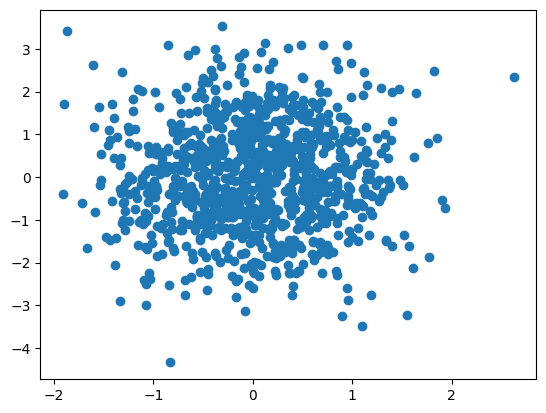
evd = la.eig(Sigma_hat)
lambda_ = evd[0]
v_hat = evd[1]
u_hat = np.matmul(X, np.transpose(v_hat))
plt.scatter(u_hat[:,0], u_hat[:,1]);

_images/2c0e0c77af9985ef7cb2cad187bfc8f452de1b52ca5b0c5227a97e606f2a1480.png

Fit using scikitlearn’s function

pca = PCA(n_components = 2).fit(X)
print(pca.explained_variance_)
print(lambda_ )

[1.53513079 0.48405623]
[1.53513079 0.48405623]

Example#

Let’s consider the melanoma dataset that we looked at before. First we read in the data as we have done before so we don’t show that code.

#| echo: false
data_flag = 'dermamnist'

## This defines our NN parameters
NUM_EPOCHS = 10
BATCH_SIZE = 128
lr = 0.001

info = INFO[data_flag]
task = info['task']
n_channels = info['n_channels']
n_classes = len(info['label'])

##https://github.com/MedMNIST/MedMNIST/blob/main/examples/getting_started.ipynb
data_flag = 'dermamnist'

data_transform = transforms.Compose([

  transforms.ToTensor()

])
DataClass = getattr(medmnist, info['python_class'])

# load the data
train_dataset = DataClass(split = 'train', transform = data_transform, download = True)
test_dataset  = DataClass(split = 'test' , transform = data_transform, download = True)
pil_dataset   = DataClass(split = 'train',                             download = True)

train_loader = data.DataLoader(dataset=train_dataset, batch_size=BATCH_SIZE, shuffle=True)
test_loader = data.DataLoader(dataset=test_dataset, batch_size=2*BATCH_SIZE, shuffle=False)

Downloading https://zenodo.org/records/10519652/files/dermamnist.npz?download=1 to /root/.medmnist/dermamnist.npz

100%|██████████| 19725078/19725078 [00:02<00:00, 9532838.96it/s]

Using downloaded and verified file: /root/.medmnist/dermamnist.npz
Using downloaded and verified file: /root/.medmnist/dermamnist.npz

Next, let’s get the data from the torch dataloader format back into an image array and a matrix with the image part (28, 28, 3) vectorized.

def loader_to_array(dataloader):
  ## Read one iteration to get data
  test_input, test_target = next(iter(dataloader))
  ## Total number of training images
  n = np.sum([inputs.shape[0] for inputs, targets in dataloader])
  ## The dimensions of the images
  imgdim = (test_input.shape[2], test_input.shape[3])
  images = np.empty( (n, imgdim[0], imgdim[1], 3))

  ## Read the data from the data loader into our numpy array
  idx = 0
  for inputs, targets in dataloader:
    inputs = inputs.detach().numpy()
    for j in range(inputs.shape[0]):
      img = inputs[j,:,:,:]
      ## get it out of pytorch format
      img = np.transpose(img, (1, 2, 0))
      images[idx,:,:,:] = img
      matrix = images.reshape(n, 3 * np.prod(imgdim))
      idx += 1
  return images, matrix

train_images, train_matrix = loader_to_array(train_loader)
test_images, test_matrix = loader_to_array(test_loader)

## Demean the matrices
train_mean = train_matrix.mean(0)
train_matrix = train_matrix - train_mean
test_mean = test_matrix.mean(0)
test_matrix = test_matrix - test_mean

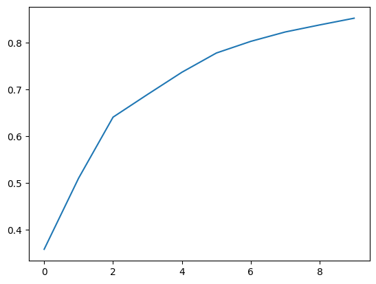
Now let’s actually perform PCA using scikitlearn. We’ll plot the eigenvalues divided by their sums, $λ_{k} / \sum_{k^{'}} λ_{k^{'}}$ . This is called a scree plot.

from sklearn.decomposition import PCA
n_comp = 10
pca = PCA(n_components = n_comp).fit(train_matrix)
plt.plot(pca.explained_variance_ratio_);

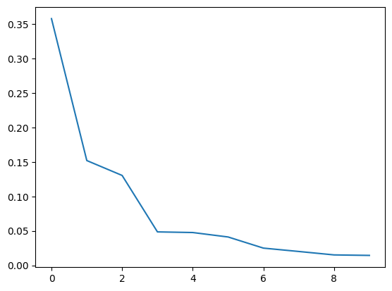
_images/72cf9790cf04f702b7cf5a28d26546b262c9fd27b7abf9203ce783aa3065b6ee.png

Often this is done by plotting the cummulative sum so that you can visualize how much variance is explained by including the top $k$ components. Here I fit 10 components and they explain 85% of the variation.

plt.plot(np.cumsum(pca.explained_variance_ratio_));

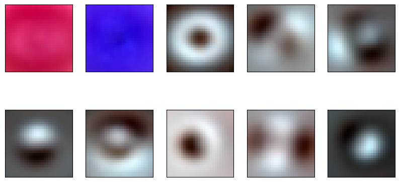
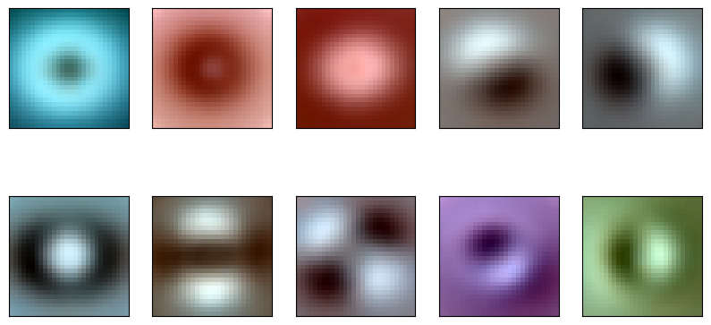
_images/55fc4ea67ddb30c1f1971fdcae9c1de35d6beb5c5e12b7fa1093233271ce6af3.png

Note that the weights from the eigenvectors, $V$ , are images. We can plot these as images.

eigen_moles = pca.components_

#| echo: false
plt.figure(figsize=(10,5))
for i in range(10):
  plt.subplot(2, 5,i+1)
  plt.xticks([])
  plt.yticks([])
  img = eigen_moles[i,:].reshape(28, 28, 3)
  img = (img - img.min())
  img = img / img.max()
  img = img * 255
  img = img.astype(np.uint8)
  plt.imshow(img)

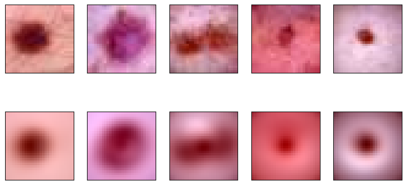
_images/9c526dfaab02d72b8f8b6ca078e00b0e8ec6af1f83534e45de8619a80a082054.png

Let’s project our testing data onto the principal component basis created by our training data and see how it does. Let $X_{t r a i n i n g} = U Λ^{1 / 2} V^{t}$ is the SVD of our training data. Then, we can convert ths scores, $U$ back to $X_{t r a i n i n g}$ with the map $U \to U λ^{1 / 2} V$ . Or, if our scores are normalized, $U Λ^{1 / 2}$ then we simply multiply by $V^{t}$ . If we want to represent $X_{t r a i n i n g}$ by a lower dimensional summary, we just keep fewer columns of scores, then multiply by the same columns of $V$ . We could write this as $U_{s} = X_{t r a i n i n g} V_{S} λ_{S}^{- 1 / 2}$ , where $S$ refers to a subset of values of $k$ .

Notice that ${\hat{X}}_{t r a i n i n g} = U_{S} V_{S}^{t} Λ_{S}^{- 1 / 2} = X_{t r a i n i n g} V_{S} V_{S}^{t}$ , $Λ$ and $V$ . Consider then an approximation to $X_{t e s t}$ as ${\hat{X}}_{t e s t} = X_{t e s t} V_{s} V_{S}^{t}$ . Written otherwise $ ${\hat{X}}_{i, t e s t} = \sum_{k \in S} < x_{i, t e s t}, v_{k} > v_{k}$ $w h i c h i s t h e p r o j e c t i o n o f s u b j e c t$ i$’s features into the linear space spanned by the basis defined by the principal component loadings.

Let’s try this on our mole data.

test_matrix_fit = pca.inverse_transform(pca.transform(test_matrix))
np.mean(np.abs( test_matrix - test_matrix_fit))

0.03792390874027308

#| echo: false
test_matrix_fit_remeaned = test_matrix_fit + test_mean
test_matrix_remeaned = test_matrix + test_mean

plt.figure(figsize=(10,5))
for i in range(5):
  plt.subplot(2, 5,i+1)
  plt.xticks([])
  plt.yticks([])
  img = test_matrix_remeaned[i,:].reshape(28, 28, 3)
  img = (img - img.min())
  img = img / img.max()
  img = img * 255
  img = img.astype(np.uint8)
  plt.imshow(img)

  plt.subplot(2, 5,i+6)
  plt.xticks([])
  plt.yticks([])
  img = test_matrix_fit_remeaned[i,:].reshape(28, 28, 3)
  img = (img - img.min())
  img = img / img.max()
  img = img * 255
  img = img.astype(np.uint8)
  plt.imshow(img)

_images/1b6e0f33449bb1ad3ab8b3f9d7b48a4a3f919f36463c9c6b4a4ee83edf375c3b.png

ICA#

ICA, independent components analysis, tries to find linear transformations of the data that are statistically independent. Usually, independence is an assumption in ICA, not actually embedded in the loss function.

Let $S_{t}$ be an $R^{p}$ collection of $p$ source signals. Assume that the underlying signals are independent, so that $S_{t} \sim F = F_{1} \times F_{2} \times \dots \time f_{p}$ . Assume that the observed data is $X_{t} = M S_{t}$ and $X_{t} \sim G$ . It is typically assumed that $M$ is invertible so that $S_{t} = M^{- 1} X_{t}$ and $M$ and $M^{- 1}$ are called the mixing and unmixing matrices respectively. Note that, since we observe $X_{t}$ over many repititions of $t$ , we can get an estimate of $G$ . Typically, it is also assumed that the $X_{t}$ are iid over $t$ .

One way to characterize the estimation problem is to parameterize $F_{1}$ , $F_{2}$ and $F_{3}$ and use maximum likelihood, or equivalent [citations]. Another is to minimize some distance between $G$ and $F_{1}$ , $F_{2}$ and $F_{3}$ . Yet another is to actually maximize independence between the components of $S_{t}$ using some estimate of independence [cite Matteson].

The most popular approaches try to find $M^{- 1}$ by maximizing non-Gaussianity. The logic goes that 1) interesting features tend to be non-Gaussian and 2) an appeal to the CLT over signals suggest that the mixed signals should be more Gaussian by being linear combinations of independent things. The latter claim is heuristic relative to the formal CLT. However, maximizing non-Gaussian components tends to work well in practice, thus validating the motivation empirically.

One form of ICA maximizes the kurtosis. If $Y$ is a random variable, then $E [Y^{4}] - 3 E [Y^{2}]$ is the kurtosis. One could then find $M^{- 1}$ that maximizes the empirical kurtosis of the unmixed signals. Another variation of non-Gaussianity maximizes neg-entropy. The neg-entropy of a density $h$ is given by $$

\int h(y) \log(h(y)) dy = - E_h[\log h(Y)] $ $A w e l l k n o w n t h e o r e m s t a t e s t h a t t h e G a u s s i a n d i s t r i b u t i o n h a s t h e l a r g e s t e n t r o p y o f a l l d i s t r i b u t i o n s w i t h t h e s a m e v a r i a n c e . T h e r e f o r e, t o m a x i m i z e n o n - G a u s s i a n i t y, w e c a n m i n m i z e e n t r o p y, o r e q u i v a l e n t l y m a x i m i z e n e g - e n t r o p y . W e c o u l d s u b t r a c t t h e e n t r o p y o f t h e G a u s s i a n d i s t r i b u t i o n t o c o n s i d e r t h i s a c r o s s e n t r o p y p r o b l e m, b u t t h a t o n l y a d d s a c o n s t a n t t o t h e l o s s f u n c t i o n . T h e m a x i m i z a t i o n o f n e g - e n t r o p y c a n b e d o n e m a n y w a y s . W e n e e d t h e f o l l o w i n g . F o r a g i v e n$ M^{-1} $, e s t i m a t e$ G $f r o m t h e c o l l e c t i o n$ M^{-1} X_t $, t h e n c a l c u l a t e t h e n e g - e n t r o p y o f$ f_j $. U s e t h a t t o t h e n t a k e a n o p i m i z a t i o n s t e p o f$ M $i s t h e r i g h t d i r e c t i o n . S o m e v e r s i o n s o f e s t i m a t i o n u s e a p o l y n o m i a l e x p a n s i o n o f t h e$ f_j$, which then typically only requires higher order moments, like kurtosis. Fast ICA is a particular implmementation of maximizing neg-entropy.

Statistical versions of ICA don’t require $M$ to be invertible. Moreover, error terms can be added in which case you can see the connection between ICA and factor analytic models. However, factor analysis models tend to assume Gaussianity.

Example#

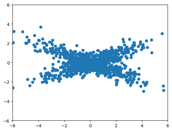
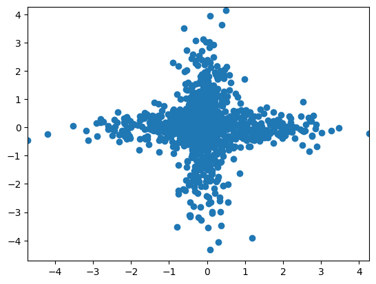
Consider an example that PCA would have somewhat of a hard time with. In this case, our data is from a mixture of normals with half from a normal with a strong positive correlation and half with a strong negative correlation. Because the angle between the two is not 90 degrees PCA has no chance. No rotation of the axes satisfies the obvious structure in this data.

n = 1000

Sigma = np.array([[4, 1.8], [1.8, 1]])
a = np.random.multivariate_normal( mean = [0, 0], cov = Sigma, size = int(n/2))
Sigma = np.array([[4, -1.8], [-1.8, 1]])
b = np.random.multivariate_normal( mean = [0, 0], cov = Sigma, size = int(n/2))
x = np.append( a, b, axis = 0)
plt.scatter(x[:,0], x[:,1])
plt.xlim([-6, 6])
plt.ylim([-6, 6])

(-6.0, 6.0)

_images/bc626f0c9b4d584fe7b6d7f9ab872ae3181f19cb774bc5b48f1266d07519ce68.png

Let’s try fast ICA. Notice it comes much closer to discovering the structure we’d like to discover than PCA could. It pulls appart the two components to a fair degree. Also note, there’s a random starting point of ICA, so that I get fairly different fits over re-runs of the algorithm. I had to lower the tolerance to get a good fit.

Indpendent components are order invariant and sign invariant.

transformer = FastICA(tol = 1e-7)
icafit = transformer.fit(x)
s = icafit.transform(x)
plt.scatter(s[:,0], s[:,1])
plt.xlim( [s.min(), s.max()])
plt.ylim( [s.min(), s.max()])

/usr/local/lib/python3.10/dist-packages/sklearn/decomposition/_fastica.py:128: ConvergenceWarning: FastICA did not converge. Consider increasing tolerance or the maximum number of iterations.
  warnings.warn(

(-4.7190845526356995, 4.268426740921572)

_images/6d35d871b52d005c014b68ea171babafb6b248a6e5875868ba6202a04eebf8b0.png

Cocktail party example#

The classic ICA problem is the so called cocktail party problem. In this, you have $p$ sources and $p$ microphones. The microphones each pick up a mixture of signals from the different sources. The goal is to unmix the sources into the components. Independence makes sense in the cocktail party example, since logically conversations would have some independence.

## If you need to get the files if running on colab this
## puts them in the same relative spot as the github directory
#!mkdir assetts
#!mkdir assetts/mp3s
#%cd assetts/mp3s
#!wget https://github.com/smart-stats/ds4bio_book/raw/refs/heads/main/book/assetts/mp3s/4.mp3 &> /dev/null
#!wget https://github.com/smart-stats/ds4bio_book/raw/refs/heads/main/book/assetts/mp3s/2.mp3 &> /dev/null
#!wget https://github.com/smart-stats/ds4bio_book/raw/refs/heads/main/book/assetts/mp3s/6.mp3 &> /dev/null
#%cd ../..

## So annoying, I misspelled assets but now there's too many things linking
## to it to change
s1, i1 = a2n.audio_from_file("assetts/mp3s/4.mp3")
s2, i2 = a2n.audio_from_file("assetts/mp3s/2.mp3")
s3, i3 = a2n.audio_from_file("assetts/mp3s/6.mp3")

## Get everything to be the same shape and sum the two audio channels
n = np.min((s1.shape[0], s2.shape[0], s3.shape[0]))
s1 = s1[0:n,:].mean(axis = 1)
s2 = s2[0:n,:].mean(axis = 1)
s3 = s3[0:n,:].mean(axis = 1)

s = np.array([s1, s2, s3])

#| echo: false
IPython.display.Audio(s1, rate = i1)

#| echo: false
IPython.display.Audio(s2, rate = i1)

#| echo: false
IPython.display.Audio(s3, rate = i1)

Mix the signals.

w = np.array( [ [.7, .2, .1], [.1, .7, .2], [.2, .1, .7] ])
x = np.transpose(np.matmul(w, s))

Here’s an example mixed signal

IPython.display.Audio(data = x[:,1].reshape(n), rate = i1)

Now try to unmix using fastICA

transformer = FastICA(whiten='unit-variance', tol = 1e-7)
icafit = transformer.fit(x)

icafit.mixing_

Unmixing matrix

icafit.components_

array([[14.83234064, -4.14317395, -1.06280459],
       [-1.8715552 , -0.32901438,  6.94242909],
       [-1.18667626, 17.11366031, -4.77739855]])

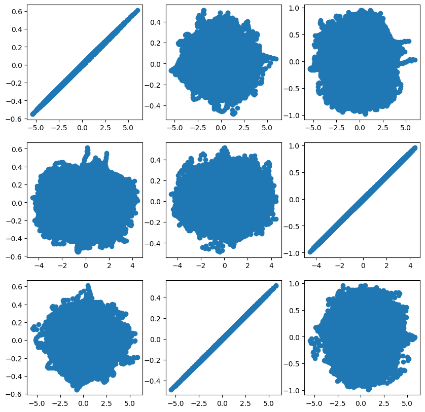
Here’s a scatterplot matrix where the real component is on the rows and the estimated component is on the columns.

hat_s = np.transpose(icafit.transform(x))

plt.figure(figsize=(10,10))

for i in range(3):
  for j in range(3):
    plt.subplot(3, 3, (3 * i + j) + 1)
    plt.scatter(hat_s[i,:].squeeze(), np.asarray(s)[j,:])

_images/af6158ea96b1a7e6d6ef950212881170ebfaf49f67dfcbddfc062bc9ba67530d.png

We can now play the estimated sources and see how they turned out.

from scipy.io.wavfile import write
i = 0
data = (hat_s[i,:].reshape(n) / np.max(np.abs(hat_s[i,:]))) * .5
IPython.display.Audio(data = data, rate = i1)

i = 1
data = (hat_s[i,:].reshape(n) / np.max(np.abs(hat_s[i,:]))) * .5
IPython.display.Audio(data = data, rate = i1)

i = 2
data = (hat_s[i,:].reshape(n) / np.max(np.abs(hat_s[i,:]))) * .5
IPython.display.Audio(data = data, rate = i1)

Imaging example using ICA#

Let’s see what we get for the images. Logically, one would consider voxels as mixed sources and images as the iid replications. But, then the sources would not be images. Let’s try the other dimension and see what we get where subject images are mixtures of source images. This is analogous to finding a soure basis of subject images.

This is often done in ICA where people transpose matrices to investigate different problems.

transformer = FastICA(n_components=10, random_state=0,whiten='unit-variance', tol = 1e-7)
icafit = transformer.fit_transform(np.transpose(train_matrix))
icafit.shape

/usr/local/lib/python3.10/dist-packages/sklearn/decomposition/_fastica.py:128: ConvergenceWarning: FastICA did not converge. Consider increasing tolerance or the maximum number of iterations.
  warnings.warn(

(2352, 10)

#| echo: false

train_matrix_remeaned = train_matrix + train_mean

plt.figure(figsize=(10,5))
for i in range(10):
  plt.subplot(2, 5,i+1)
  plt.xticks([])
  plt.yticks([])
  img = icafit[:,i].reshape(28, 28, 3)
  img = (img - img.min())
  img = img / img.max()
  img = img * 255
  img = img.astype(np.uint8)
  plt.imshow(img)

_images/227426a3fdfde5ceadc663103ec5376f02fbf1322c2e9e1066faa81e7b9e274a.png

Unsupervised learning

Contents

Unsupervised learning#

PCA#

Sample PCA#

PCA with a large dimension#

Simple example#

Example#

ICA#

Example#

Cocktail party example#

Imaging example using ICA#